Fits SVM with variable selection using penalties.
svmfs.RdFits SVM with variable selection (clone selection) using penalties SCAD, L1 norm, Elastic Net (L1 + L2 norms) and ELastic SCAD (SCAD + L1 norm). Additionally tuning parameter search is presented by two approcaches: fixed grid or interval search. NOTE: The name of the function has been changed: svmfs instead of svm.fs!
Usage
# Default S3 method
svmfs(x,y,
        fs.method = c("scad", "1norm", "scad+L2", "DrHSVM"),
        grid.search=c("interval","discrete"),
        lambda1.set=NULL,
        lambda2.set=NULL,
        bounds=NULL,
        parms.coding= c("log2","none"),
        maxevals=500,
        inner.val.method = c("cv", "gacv"),
        cross.inner= 5,
        show= c("none", "final"),
        calc.class.weights=FALSE,
        class.weights=NULL,
        seed=123,
        maxIter=700,
        verbose=TRUE,
        ...)
Arguments
- x
input matrix with genes in columns and samples in rows!
- y
numerical vector of class labels, -1 , 1
- fs.method
feature selection method. Availible 'scad', '1norm' for 1-norm, "DrHSVM" for Elastic Net and "scad+L2" for Elastic SCAD
- grid.search
chose the search method for tuning lambda1,2: 'interval' or 'discrete', default: 'interval'
- lambda1.set
for fixed grid search: fixed grid for lambda1, default: NULL
- lambda2.set
for fixed grid search: fixed grid for lambda2, default: NULL
- bounds
for interval grid search: fixed grid for lambda2, default: NULL
- parms.coding
for interval grid search: parms.coding: none or log2 , default: log2
- maxevals
the maximum number of DIRECT function evaluations, default: 500.
- calc.class.weights
calculate class.weights for SVM, default: FALSE
- class.weights
a named vector of weights for the different classes, used for asymetric class sizes. Not all factor levels have to be supplied (default weight: 1). All components have to be named.
- inner.val.method
method for the inner validation: cross validation, gacv , default cv
- cross.inner
'cross.inner'-fold cv, default: 5
- show
for interval search: show plots of DIRECT algorithm: none, final iteration, all iterations. Default: none
- seed
seed
- maxIter
maximal iteration, default: 700
- verbose
verbose?, default: TRUE
- ...
additional argument(s)
Details
The goodness of the model is highly correlated with the choice of tuning parameter lambda. Therefore the model is trained with different lambdas and the best model with optimal tuning parameter is used in futher analysises. For very small lamdas is recomended to use maxIter, otherweise the algorithms is slow or might not converge.
The Feature Selection methods are using different techniques for finding optimal tunung parameters By SCAD SVM Generalized approximate cross validation (gacv) error is calculated for each pre-defined tuning parameter.
By L1-norm SVM the cross validation (default 5-fold) missclassification error is calculated for each lambda. After training and cross validation, the optimal lambda with minimal missclassification error is choosen, and a final model with optimal lambda is created for the whole data set.
Value
- classes
vector of class labels as input 'y'
- sample.names
sample names
- class.method
feature selection method
- seed
seed
- model
final model
w - coefficients of the hyperplane
b - intercept of the hyperplane
xind - the index of the selected features (genes) in the data matrix.
index - the index of the resulting support vectors in the data matrix.
type - type of svm, from svm function
lam.opt - optimal lambda
gacv - corresponding gacv
References
Becker, N., Werft, W., Toedt, G., Lichter, P. and Benner, A.(2009) PenalizedSVM: a R-package for feature selection SVM classification, Bioinformatics, 25(13),p 1711-1712
Author
Natalia Becker
natalie_becker@gmx.de
See also
predict.penSVM, svm (in package e1071)
Examples
# \donttest{
seed<- 123
train<-sim.data(n = 200, ng = 100, nsg = 10, corr=FALSE, seed=seed )
print(str(train))
#> List of 3
#> $ x : num [1:100, 1:200] 0.547 0.635 -0.894 0.786 2.028 ...
#> ..- attr(*, "dimnames")=List of 2
#> .. ..$ : chr [1:100] "pos1" "pos2" "pos3" "pos4" ...
#> .. ..$ : chr [1:200] "1" "2" "3" "4" ...
#> $ y : Named num [1:200] 1 -1 -1 1 -1 -1 1 -1 -1 -1 ...
#> ..- attr(*, "names")= chr [1:200] "1" "2" "3" "4" ...
#> $ seed: num 123
#> NULL
### Fixed grid ####
# train SCAD SVM ####################
# define set values of tuning parameter lambda1 for SCAD
lambda1.scad <- c (seq(0.01 ,0.05, .01), seq(0.1,0.5, 0.2), 1 )
# for presentation don't check all lambdas : time consuming!
lambda1.scad<-lambda1.scad[2:3]
#
# train SCAD SVM
# computation intensive; for demostration reasons only for the first 100 features
# and only for 10 Iterations maxIter=10, default maxIter=700
system.time(scad.fix<- svmfs(t(train$x)[,1:100], y=train$y, fs.method="scad",
cross.outer= 0, grid.search = "discrete",
lambda1.set=lambda1.scad,
parms.coding = "none", show="none",
maxIter = 10, inner.val.method = "cv", cross.inner= 5,
seed=seed, verbose=FALSE) )
#> [1] "grid search"
#> [1] "discrete"
#> [1] "show"
#> [1] "none"
#> [1] "feature selection method is scad"
#> List of 2
#> $ :List of 2
#> ..$ q.val: num 0.305
#> ..$ model:List of 10
#> .. ..$ w : Named num [1:72] 0.692 0.587 1.214 0.765 0.889 ...
#> .. .. ..- attr(*, "names")= chr [1:72] "pos1" "pos2" "pos3" "pos4" ...
#> .. ..$ b : num 0.0334
#> .. ..$ xind : int [1:72] 1 2 3 4 5 6 7 8 9 10 ...
#> .. ..$ index : int [1:84] 4 16 20 33 46 47 48 58 59 64 ...
#> .. ..$ fitted : num [1:200] 8.41 -1.48 -1.01 1.25 -8.75 ...
#> .. ..$ type : num 0
#> .. ..$ lambda1 : num 0.02
#> .. ..$ iter : num 10
#> .. ..$ q.val : num 0.305
#> .. ..$ inner.val.method: chr "cv"
#> ..- attr(*, "class")= chr "penSVM"
#> $ :List of 2
#> ..$ q.val: num 0.3
#> ..$ model:List of 10
#> .. ..$ w : Named num [1:66] 0.675 0.632 1.182 0.803 0.934 ...
#> .. .. ..- attr(*, "names")= chr [1:66] "pos1" "pos2" "pos3" "pos4" ...
#> .. ..$ b : num 0.0295
#> .. ..$ xind : int [1:66] 1 2 3 4 5 6 7 8 9 10 ...
#> .. ..$ index : int [1:84] 4 16 20 33 46 47 48 58 59 64 ...
#> .. ..$ fitted : num [1:200] 8.43 -1.54 -1.02 1.36 -8.94 ...
#> .. ..$ type : num 0
#> .. ..$ lambda1 : num 0.03
#> .. ..$ iter : num 10
#> .. ..$ q.val : num 0.3
#> .. ..$ inner.val.method: chr "cv"
#> ..- attr(*, "class")= chr "penSVM"
#> NULL
#> List of 10
#> $ w : Named num [1:66] 0.675 0.632 1.182 0.803 0.934 ...
#> ..- attr(*, "names")= chr [1:66] "pos1" "pos2" "pos3" "pos4" ...
#> $ b : num 0.0295
#> $ xind : int [1:66] 1 2 3 4 5 6 7 8 9 10 ...
#> $ index : int [1:84] 4 16 20 33 46 47 48 58 59 64 ...
#> $ fitted : num [1:200] 8.43 -1.54 -1.02 1.36 -8.94 ...
#> $ type : num 0
#> $ lambda1 : num 0.03
#> $ iter : num 10
#> $ q.val : num 0.3
#> $ inner.val.method: chr "cv"
#> NULL
#> user system elapsed
#> 0.375 0.014 0.390
print(scad.fix)
#>
#> Bias =
#> Selected Variables=
#> Coefficients:
#> NULL
#>
# train 1NORM SVM ################
# define set values of tuning parameter lambda1 for 1norm
#epsi.set<-vector(); for (num in (1:9)) epsi.set<-sort(c(epsi.set,
# c(num*10^seq(-5, -1, 1 ))) )
## for presentation don't check all lambdas : time consuming!
#lambda1.1norm <- epsi.set[c(3,5)] # 2 params
#
### train 1norm SVM
## time consuming: for presentation only for the first 100 features
#norm1.fix<- svmfs(t(train$x)[,1:100], y=train$y, fs.method="1norm",
# cross.outer= 0, grid.search = "discrete",
# lambda1.set=lambda1.1norm,
# parms.coding = "none", show="none",
# maxIter = 700, inner.val.method = "cv", cross.inner= 5,
# seed=seed, verbose=FALSE )
#
# print(norm1.fix)
### Interval search ####
seed <- 123
train<-sim.data(n = 200, ng = 100, nsg = 10, corr=FALSE, seed=seed )
print(str(train))
#> List of 3
#> $ x : num [1:100, 1:200] 0.547 0.635 -0.894 0.786 2.028 ...
#> ..- attr(*, "dimnames")=List of 2
#> .. ..$ : chr [1:100] "pos1" "pos2" "pos3" "pos4" ...
#> .. ..$ : chr [1:200] "1" "2" "3" "4" ...
#> $ y : Named num [1:200] 1 -1 -1 1 -1 -1 1 -1 -1 -1 ...
#> ..- attr(*, "names")= chr [1:200] "1" "2" "3" "4" ...
#> $ seed: num 123
#> NULL
test<-sim.data(n = 200, ng = 100, nsg = 10, corr=FALSE, seed=seed+1 )
print(str(test))
#> List of 3
#> $ x : num [1:100, 1:200] 1.07 1.02 1.89 1.65 -1.19 ...
#> ..- attr(*, "dimnames")=List of 2
#> .. ..$ : chr [1:100] "pos1" "pos2" "pos3" "pos4" ...
#> .. ..$ : chr [1:200] "1" "2" "3" "4" ...
#> $ y : Named num [1:200] 1 -1 -1 -1 -1 1 -1 1 -1 -1 ...
#> ..- attr(*, "names")= chr [1:200] "1" "2" "3" "4" ...
#> $ seed: num 124
#> NULL
bounds=t(data.frame(log2lambda1=c(-10, 10)))
colnames(bounds)<-c("lower", "upper")
# computation intensive; for demostration reasons only for the first 100 features
# and only for 10 Iterations maxIter=10, default maxIter=700
print("start interval search")
#> [1] "start interval search"
system.time( scad<- svmfs(t(train$x)[,1:100], y=train$y,
fs.method="scad", bounds=bounds,
cross.outer= 0, grid.search = "interval", maxIter = 10,
inner.val.method = "cv", cross.inner= 5, maxevals=500,
seed=seed, parms.coding = "log2", show="none", verbose=FALSE ) )
#> [1] "grid search"
#> [1] "interval"
#> [1] "show"
#> [1] "none"
#> [1] "feature selection method is scad"
#> Warning: Coercing LHS to a list
#> Warning: Coercing LHS to a list
#> Warning: Coercing LHS to a list
#> Warning: Coercing LHS to a list
#> Warning: Coercing LHS to a list
#> Warning: Coercing LHS to a list
#> Warning: Coercing LHS to a list
#> Warning: Coercing LHS to a list
#> Warning: Coercing LHS to a list
#> Warning: Coercing LHS to a list
#> Warning: Coercing LHS to a list
#> ...done
#> ...done
#> ...done
#> ...done
#> ...done
#> ...done
#> ...done
#> ...done
#> ...done
#> ...done
#> ...done
#> ...done
#> ...done
#> ...done
#> ...done
#> ...done
#> ...done
#> ...done
#> ...done
#> ...done
#> ...done
#> ...done
#> ...done
#> ...done
#> ...done
#> ...done
#> ...done
#> ...done
#> ...done
#> ...done
#> ...done
#> ...done
#> ...done
#> ...done
#> ...done
#> ...done
#> ...done
#> ...done
#> ...done
#> ...done
#> ...done
#> ...done
#> ...done
#> ...done
#> ...done
#> ...done
#> ...done
#> ...done
#> ...done
#> ...done
#> ...done
#> ...done
#> ...done
#> ...done
#> ...done
#> ...done
#> ...done
#> ...done
#> ...done
#> ...done
#> ...done
#> ...done
#> ...done
#> ...done
#> ...done
#> ...done
#> ...done
#> ...done
#> ...done
#> ...done
#> ...done
#> ...done
#> ...done
#> ...done
#> ...done
#> ...done
#> ...done
#> ...done
#> ...done
#> ...done
#> user system elapsed
#> 6.004 0.128 6.161
print("scad final model")
#> [1] "scad final model"
print(str(scad$model))
#> List of 11
#> $ w : Named num [1:22] 0.444 0.693 0.835 0.863 0.587 ...
#> ..- attr(*, "names")= chr [1:22] "pos1" "pos2" "pos3" "pos4" ...
#> $ b : num -0.0229
#> $ xind : int [1:22] 1 2 3 4 5 6 7 8 9 10 ...
#> $ index : int [1:84] 4 16 20 33 46 47 48 58 59 64 ...
#> $ fitted : num [1:200] 1.946 -0.873 -1.704 0.915 -5.617 ...
#> $ type : num 0
#> $ lambda1 : num 0.122
#> $ lambda2 : NULL
#> $ iter : num 10
#> $ q.val : num 0.185
#> $ fit.info:List of 13
#> ..$ fmin : num 0.185
#> ..$ xmin : Named num -3.04
#> .. ..- attr(*, "names")= chr "log2lambda1"
#> ..$ iter : num 17
#> ..$ neval : num 37
#> ..$ maxevals : num 500
#> ..$ seed : num 123
#> ..$ bounds : num [1, 1:2] -10 10
#> .. ..- attr(*, "dimnames")=List of 2
#> .. .. ..$ : chr "log2lambda1"
#> .. .. ..$ : chr [1:2] "lower" "upper"
#> ..$ Q.func : chr ".calc.scad"
#> ..$ points.fmin:'data.frame': 1 obs. of 2 variables:
#> .. ..$ log2lambda1: num -3.04
#> .. ..$ f : num 0.185
#> ..$ Xtrain : num [1:37, 1] 1.532 -1.338 -0.435 -8.453 3.531 ...
#> .. ..- attr(*, "dimnames")=List of 2
#> .. .. ..$ : NULL
#> .. .. ..$ : chr "log2lambda1"
#> ..$ Ytrain : num [1:37] 1.00e+16 4.65e-01 1.00e+16 3.05e-01 1.00e+16 ...
#> ..$ gp.seed : num [1:16] 123 124 125 126 127 128 129 130 131 132 ...
#> ..$ model.list :List of 1
#> .. ..$ model:List of 10
#> .. .. ..$ w : Named num [1:22] 0.444 0.693 0.835 0.863 0.587 ...
#> .. .. .. ..- attr(*, "names")= chr [1:22] "pos1" "pos2" "pos3" "pos4" ...
#> .. .. ..$ b : num -0.0229
#> .. .. ..$ xind : int [1:22] 1 2 3 4 5 6 7 8 9 10 ...
#> .. .. ..$ index : int [1:84] 4 16 20 33 46 47 48 58 59 64 ...
#> .. .. ..$ fitted : num [1:200] 1.946 -0.873 -1.704 0.915 -5.617 ...
#> .. .. ..$ type : num 0
#> .. .. ..$ lambda1 : num 0.122
#> .. .. ..$ iter : num 10
#> .. .. ..$ q.val : num 0.185
#> .. .. ..$ inner.val.method: chr "cv"
#> NULL
(scad.5cv.test<-predict.penSVM(scad, t(test$x)[,1:100], newdata.labels=test$y) )
#> $pred.class
#> [1] 1 -1 -1 1 -1 -1 1 1 -1 -1 1 1 -1 1 -1 1 1 1 -1 1 -1 1 -1 -1 -1
#> [26] 1 1 -1 -1 -1 1 1 1 -1 1 1 -1 -1 1 1 -1 -1 1 1 1 1 1 -1 -1 -1
#> [51] 1 -1 1 1 -1 -1 -1 1 1 -1 -1 -1 -1 1 1 1 -1 -1 -1 -1 -1 -1 1 1 1
#> [76] -1 -1 -1 -1 1 1 -1 -1 1 1 1 1 1 -1 1 -1 1 -1 -1 -1 -1 1 1 1 1
#> [101] -1 -1 -1 -1 -1 1 1 -1 1 -1 1 -1 -1 -1 -1 1 1 -1 1 1 1 -1 1 -1 1
#> [126] 1 -1 -1 -1 1 -1 -1 1 1 1 1 1 -1 -1 1 1 1 1 1 1 -1 -1 1 -1 1
#> [151] 1 1 -1 -1 -1 1 -1 1 1 -1 1 -1 -1 1 -1 -1 -1 1 1 1 1 1 -1 1 1
#> [176] 1 -1 1 -1 -1 1 -1 -1 -1 -1 1 -1 1 1 1 -1 -1 -1 -1 1 1 1 1 1 1
#> Levels: -1 1
#>
#> $fitted
#> [,1]
#> 1 2.916046876
#> 2 -0.935231697
#> 3 -1.581906448
#> 4 0.485830856
#> 5 -1.385142530
#> 6 -0.458484391
#> 7 0.413884259
#> 8 0.456234359
#> 9 -0.503227694
#> 10 -0.250689821
#> 11 0.601966924
#> 12 3.224820070
#> 13 -2.488100168
#> 14 1.513471244
#> 15 -0.272209344
#> 16 0.668590048
#> 17 2.067604880
#> 18 3.473798666
#> 19 -0.807700750
#> 20 3.314894067
#> 21 -1.351370641
#> 22 2.837563341
#> 23 -2.351475057
#> 24 -1.960668897
#> 25 -1.735973253
#> 26 0.244063538
#> 27 2.093742344
#> 28 -4.190937196
#> 29 -1.260214644
#> 30 -2.045537650
#> 31 2.428183957
#> 32 0.783898648
#> 33 3.347844389
#> 34 -3.457786474
#> 35 2.054277530
#> 36 0.162067747
#> 37 -3.545284833
#> 38 -1.688978604
#> 39 0.560941105
#> 40 0.953671030
#> 41 -1.998076531
#> 42 -2.762780838
#> 43 2.721174397
#> 44 3.495771096
#> 45 3.131833170
#> 46 0.772864321
#> 47 0.154892863
#> 48 -1.437905563
#> 49 -0.290802250
#> 50 -0.476002664
#> 51 2.318267222
#> 52 -3.670834406
#> 53 1.151385655
#> 54 3.219929268
#> 55 -4.282718887
#> 56 -0.821494519
#> 57 -0.077311627
#> 58 1.870987281
#> 59 1.701197113
#> 60 -0.965236737
#> 61 -0.757520460
#> 62 -0.215005330
#> 63 -2.408416513
#> 64 0.198124580
#> 65 0.354149277
#> 66 2.499489464
#> 67 -4.642261948
#> 68 -0.008844249
#> 69 -2.044592877
#> 70 -0.120035134
#> 71 -2.002293608
#> 72 -2.499755791
#> 73 1.081386355
#> 74 0.234378949
#> 75 5.018980466
#> 76 -5.202266101
#> 77 -0.694916346
#> 78 -2.277477884
#> 79 -1.723885624
#> 80 4.731376593
#> 81 2.560434752
#> 82 -0.967699817
#> 83 -2.572720124
#> 84 0.441050145
#> 85 0.051816687
#> 86 3.412857918
#> 87 0.971650460
#> 88 0.782261234
#> 89 -0.005433330
#> 90 1.592802109
#> 91 -0.922641846
#> 92 3.040395690
#> 93 -1.127018932
#> 94 -1.626105368
#> 95 -2.783589471
#> 96 -1.877764785
#> 97 0.052325636
#> 98 1.199135329
#> 99 2.538047051
#> 100 3.736672101
#> 101 -3.288334551
#> 102 -2.744899889
#> 103 -3.016155829
#> 104 -0.105232520
#> 105 -3.005458292
#> 106 0.949483411
#> 107 0.133492738
#> 108 -3.315399827
#> 109 3.137884265
#> 110 -5.165362343
#> 111 2.381098083
#> 112 -0.565926790
#> 113 -2.622750250
#> 114 -1.843960426
#> 115 -0.567626226
#> 116 2.240838905
#> 117 1.378637301
#> 118 -0.827005436
#> 119 0.463817022
#> 120 2.181054770
#> 121 0.123921001
#> 122 -3.505630433
#> 123 3.521699419
#> 124 -3.365547854
#> 125 2.239288004
#> 126 0.579776861
#> 127 -1.723551029
#> 128 -4.956955266
#> 129 -0.700216100
#> 130 2.319403692
#> 131 -2.049697843
#> 132 -2.552784159
#> 133 5.034438294
#> 134 0.371816904
#> 135 0.582482459
#> 136 0.120685789
#> 137 7.392134264
#> 138 -0.769002200
#> 139 -0.774195093
#> 140 1.081430185
#> 141 1.013213846
#> 142 0.636082471
#> 143 0.647231061
#> 144 1.367407382
#> 145 0.111207977
#> 146 -0.325576678
#> 147 -2.523993732
#> 148 1.521130266
#> 149 -0.942975870
#> 150 1.031394054
#> 151 1.562418529
#> 152 3.623402569
#> 153 -0.741619728
#> 154 -4.725843469
#> 155 -3.767090006
#> 156 0.660422136
#> 157 -0.241375301
#> 158 5.092143730
#> 159 2.095050718
#> 160 -2.794850572
#> 161 3.018465506
#> 162 -0.046552575
#> 163 -1.607989118
#> 164 2.494543083
#> 165 -2.325548314
#> 166 -2.793950076
#> 167 -0.130349805
#> 168 1.284625784
#> 169 2.712990582
#> 170 1.146354932
#> 171 0.510047215
#> 172 1.658877820
#> 173 -2.220410518
#> 174 0.957441384
#> 175 0.753568611
#> 176 0.769629667
#> 177 -2.856816523
#> 178 0.497216905
#> 179 -0.730031442
#> 180 -4.704120965
#> 181 0.819667495
#> 182 -0.044115410
#> 183 -1.464921985
#> 184 -0.588958651
#> 185 -3.646403025
#> 186 1.827708859
#> 187 -0.035275303
#> 188 3.656463470
#> 189 2.335816788
#> 190 0.046067998
#> 191 -2.896973362
#> 192 -1.367408963
#> 193 -0.197043939
#> 194 -3.603519404
#> 195 1.367878486
#> 196 1.712283829
#> 197 3.799085441
#> 198 0.704499498
#> 199 1.947499243
#> 200 2.272641204
#>
#> $tab
#> newdata.labels
#> pred.class -1 1
#> -1 85 12
#> 1 26 77
#>
#> $error
#> [1] 0.19
#>
#> $sensitivity
#> [1] 0.8651685
#>
#> $specificity
#> [1] 0.7657658
#>
print(paste("minimal 5-fold cv error:", scad$model$fit.info$fmin,
"by log2(lambda1)=", scad$model$fit.info$xmin))
#> [1] "minimal 5-fold cv error: 0.185 by log2(lambda1)= -3.03520543316445"
print(" all lambdas with the same minimum? ")
#> [1] " all lambdas with the same minimum? "
print(scad$model$fit.info$ points.fmin)
#> log2lambda1 f
#> 27 -3.035205 0.185
print(paste(scad$model$fit.info$neval, "visited points"))
#> [1] "37 visited points"
print(" overview: over all visitied points in tuning parameter space
with corresponding cv errors")
#> [1] " overview: over all visitied points in tuning parameter space \n\t\twith corresponding cv errors"
print(data.frame(Xtrain=scad$model$fit.info$Xtrain,
cv.error=scad$model$fit.info$Ytrain))
#> log2lambda1 cv.error
#> 1 1.5315485 1.00e+16
#> 2 -1.3383552 4.65e-01
#> 3 -0.4348424 1.00e+16
#> 4 -8.4531580 3.05e-01
#> 5 3.5310332 1.00e+16
#> 6 -2.1035852 2.45e-01
#> 7 9.1782694 1.00e+16
#> 8 2.3956101 1.00e+16
#> 9 8.4905937 1.00e+16
#> 10 -3.7667024 2.85e-01
#> 11 -6.4618650 3.00e-01
#> 12 5.4976793 1.00e+16
#> 13 -5.3380199 2.80e-01
#> 14 1.2415551 1.00e+16
#> 15 6.7099483 1.00e+16
#> 16 -4.4249049 2.95e-01
#> 17 4.6509131 1.00e+16
#> 18 7.3355014 1.00e+16
#> 19 -7.8173000 3.05e-01
#> 20 -9.0531639 3.05e-01
#> 21 -2.7058843 2.05e-01
#> 22 -4.8506733 3.20e-01
#> 23 -9.7038186 3.00e-01
#> 24 -1.4557824 4.65e-01
#> 25 -4.2158845 2.85e-01
#> 26 -2.4017091 2.45e-01
#> 27 -3.0352054 1.85e-01
#> 28 -6.1636759 3.05e-01
#> 29 -7.1268118 2.95e-01
#> 30 -8.8040755 3.05e-01
#> 31 -5.7266564 3.05e-01
#> 32 -2.2278129 2.55e-01
#> 33 -6.8407343 3.00e-01
#> 34 -3.4158114 2.20e-01
#> 35 -8.1115934 3.05e-01
#> 36 -9.9999979 3.00e-01
#> 37 -9.4561642 3.00e-01
#
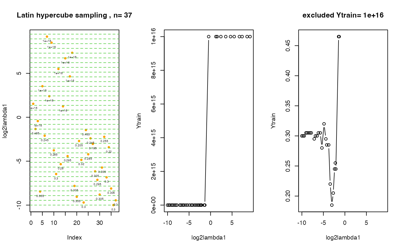
# create 3 plots on one screen:
# 1st plot: distribution of initial points in tuning parameter space
# 2nd plot: visited lambda points vs. cv errors
# 3rd plot: the same as the 2nd plot, Ytrain.exclude points are excluded.
# The value cv.error = 10^16 stays for the cv error for an empty model !
.plot.EPSGO.parms (scad$model$fit.info$Xtrain, scad$model$fit.info$Ytrain,
bound=bounds, Ytrain.exclude=10^16, plot.name=NULL )
 # } # end of \donttest