Plot Interval Search Plot Visited Points and the Q Values.

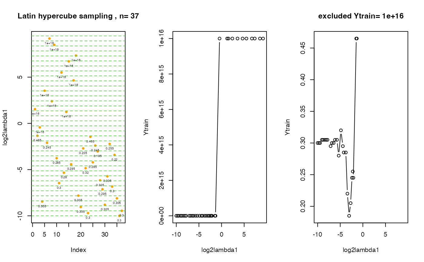
For interval search plot visited points and the Q values (=Ytrain) exclude: for D=1 make an additional plot: skip values for empty model, for example: Ytrain.exclude=10^16.

Usage

.plot.EPSGO.parms(Xtrain, Ytrain,bounds, Ytrain.exclude=10^16, plot.name=NULL )

Arguments

Xtrain

X points to train

Ytrain

Y points to train

bounds

bounds for parameters, see examples

Ytrain.exclude

If exclude for Ytrain exists, skip those points. Defaults to 10^16.

plot.name

Defaults to NULL

Value

None, only graphs are created.

Details

The code source was adopted from MATLAB originals, special thanks to Holger Froehlich.

Author

Natalia Becker
natalie_becker@gmx.de

References

Froehlich, H. and Zell, A. (2005) "Effcient parameter selection for support vector machines in classification and regression via model-based global optimization" In Proc. Int. Joint Conf. Neural Networks, 1431-1438 .

See also

svmfs

Examples

  # \donttest{
  seed <- 123
      
  train<-sim.data(n = 200, ng = 100, nsg = 10, corr=FALSE, seed=seed )
  print(str(train)) 
#> List of 3
#>  $ x   : num [1:100, 1:200] 0.547 0.635 -0.894 0.786 2.028 ...
#>   ..- attr(*, "dimnames")=List of 2
#>   .. ..$ : chr [1:100] "pos1" "pos2" "pos3" "pos4" ...
#>   .. ..$ : chr [1:200] "1" "2" "3" "4" ...
#>  $ y   : Named num [1:200] 1 -1 -1 1 -1 -1 1 -1 -1 -1 ...
#>   ..- attr(*, "names")= chr [1:200] "1" "2" "3" "4" ...
#>  $ seed: num 123
#> NULL
      
  Q.func<- ".calc.scad"
  
  bounds=t(data.frame(log2lambda1=c(-10, 10)))
              colnames(bounds)<-c("lower", "upper")  
      
  print("start interval search")
#> [1] "start interval search"
  # computation intensive; 
  # for demostration reasons only for the first 100 features 
  # and only for 10 iterations maxIter=10, default maxIter=700
  system.time(fit<-EPSGO(Q.func, bounds=bounds, parms.coding="log2", fminlower=0, 
     show='none', N=21,  maxevals=500, 
     pdf.name=NULL,  seed=seed,  
     verbose=FALSE,
     # Q.func specific parameters:
     x.svm=t(train$x)[,1:100], y.svm=train$y,
     inner.val.method="cv",
     cross.inner=5, maxIter=10 ))
#> Warning: Coercing LHS to a list
#> Warning: Coercing LHS to a list
#> Warning: Coercing LHS to a list
#> Warning: Coercing LHS to a list
#> Warning: Coercing LHS to a list
#> Warning: Coercing LHS to a list
#> Warning: Coercing LHS to a list
#> Warning: Coercing LHS to a list
#> Warning: Coercing LHS to a list
#> Warning: Coercing LHS to a list
#> Warning: Coercing LHS to a list
#> ...done
#> ...done
#> ...done
#> ...done
#> ...done
#> ...done
#> ...done
#> ...done
#> ...done
#> ...done
#> ...done
#> ...done
#> ...done
#> ...done
#> ...done
#> ...done
#> ...done
#> ...done
#> ...done
#> ...done
#> ...done
#> ...done
#> ...done
#> ...done
#> ...done
#> ...done
#> ...done
#> ...done
#> ...done
#> ...done
#> ...done
#> ...done
#> ...done
#> ...done
#> ...done
#> ...done
#> ...done
#> ...done
#> ...done
#> ...done
#> ...done
#> ...done
#> ...done
#> ...done
#> ...done
#> ...done
#> ...done
#> ...done
#> ...done
#> ...done
#> ...done
#> ...done
#> ...done
#> ...done
#> ...done
#> ...done
#> ...done
#> ...done
#> ...done
#> ...done
#> ...done
#> ...done
#> ...done
#> ...done
#> ...done
#> ...done
#> ...done
#> ...done
#> ...done
#> ...done
#> ...done
#> ...done
#> ...done
#> ...done
#> ...done
#> ...done
#> ...done
#> ...done
#> ...done
#> ...done
#>    user  system elapsed 
#>   6.042   0.125   6.199 
                   
  print(paste("minimal 5-fold cv error:", fit$fmin, "by log2(lambda1)=", fit$xmin))
#> [1] "minimal 5-fold cv error: 0.185 by log2(lambda1)= -3.03520543316445"
    
  print(" all lambdas with the same minimum? ")
#> [1] " all lambdas with the same minimum? "
  print(fit$ points.fmin) 
#>    log2lambda1     f
#> 27   -3.035205 0.185
      
  print(paste(fit$neval, "visited points"))
#> [1] "37 visited points"
      
      
  print(" overview: over all visitied points in tuning parameter space 
        with corresponding cv errors")
#> [1] " overview: over all visitied points in tuning parameter space \n\t\t\t\twith corresponding cv errors"
  print(data.frame(Xtrain=fit$Xtrain, cv.error=fit$Ytrain))
#>    log2lambda1 cv.error
#> 1    1.5315485 1.00e+16
#> 2   -1.3383552 4.65e-01
#> 3   -0.4348424 1.00e+16
#> 4   -8.4531580 3.05e-01
#> 5    3.5310332 1.00e+16
#> 6   -2.1035852 2.45e-01
#> 7    9.1782694 1.00e+16
#> 8    2.3956101 1.00e+16
#> 9    8.4905937 1.00e+16
#> 10  -3.7667024 2.85e-01
#> 11  -6.4618650 3.00e-01
#> 12   5.4976793 1.00e+16
#> 13  -5.3380199 2.80e-01
#> 14   1.2415551 1.00e+16
#> 15   6.7099483 1.00e+16
#> 16  -4.4249049 2.95e-01
#> 17   4.6509131 1.00e+16
#> 18   7.3355014 1.00e+16
#> 19  -7.8173000 3.05e-01
#> 20  -9.0531639 3.05e-01
#> 21  -2.7058843 2.05e-01
#> 22  -4.8506733 3.20e-01
#> 23  -9.7038186 3.00e-01
#> 24  -1.4557824 4.65e-01
#> 25  -4.2158845 2.85e-01
#> 26  -2.4017091 2.45e-01
#> 27  -3.0352054 1.85e-01
#> 28  -6.1636759 3.05e-01
#> 29  -7.1268118 2.95e-01
#> 30  -8.8040755 3.05e-01
#> 31  -5.7266564 3.05e-01
#> 32  -2.2278129 2.55e-01
#> 33  -6.8407343 3.00e-01
#> 34  -3.4158114 2.20e-01
#> 35  -8.1115934 3.05e-01
#> 36  -9.9999979 3.00e-01
#> 37  -9.4561642 3.00e-01

  # create  3 plots om one screen: 
  # 1st plot: distribution of initial points in tuning parameter space
  # 2nd plot: visited lambda points vs. cv errors
  # 3rd plot: the same as the 2nd plot, Ytrain.exclude points are excluded. 
  #    The value cv.error = 10^16 stays for the cv error for an empty model ! 
  .plot.EPSGO.parms (fit$Xtrain, fit$Ytrain,bound=bounds, 
        Ytrain.exclude=10^16, plot.name=NULL )

  # } # end of \donttest