Fits SVM with variable selection using penalties.
EPSGO.RdFits SVM with feature selection using penalties SCAD and 1 norm.
Arguments
- Q.func
name of the function to be minimized.
- bounds
bounds for parameters, see examples
- parms.coding
parmeters coding: none or log2, default: none.
- fminlower
minimal value for the function Q.func, default is 0.
- flag.find.one.min
do you want to find one min value and stop? Default: FALSE
- show
show plots of DIRECT algorithm: none, final iteration, all iterations. Default: none
- N
define the number of start points, see details.
- maxevals
the maximum number of DIRECT function evaluations, default: 500.
- pdf.name
pdf name
- pdf.width
default 12
- pdf.height
default 12
- my.mfrow
default c(1,1)
- verbose
verbose? default TRUE.
- seed
seed
- ...
additional argument(s)
Value
- fmin
minimal value of Q.func on the interval defined by bounds.
- xmin
coreesponding parameters for the minimum
- iter
number of iterations
- neval
number of visited points
- maxevals
the maximum number of DIRECT function evaluations
- seed
seed
- bounds
bounds for parameters
- Q.func
name of the function to be minimized.
- points.fmin
the set of points with the same fmin
- Xtrain
visited points
- Ytrain
the output of Q.func at visited points Xtrain
- gp.seed
seed for Gaussian Process
- model.list
detailed information of the search process
Details
if the number of start points (N) is not defined by the user, it will be defined dependent on the dimensionality of the parameter space. N=10D+1, where D is the number of parameters, but for high dimensional parameter space with more than 6 dimensions, the initial set is restricted to 65. However for one-dimensional parameter space the N is set to 21 due to stability reasons.
The idea of EPSGO (Efficient Parameter Selection via Global Optimization): Beginning from an intial Latin hypercube sampling containing N starting points we train an Online GP, look for the point with the maximal expected improvement, sample there and update the Gaussian Process(GP). Thereby it is not so important that GP really correctly models the error surface of the SVM in parameter space, but that it can give a us information about potentially interesting points in parameter space where we should sample next. We continue with sampling points until some convergence criterion is met.
DIRECT is a sampling algorithm which requires no knowledge of the objective function gradient. Instead, the algorithm samples points in the domain, and uses the information it has obtained to decide where to search next. The DIRECT algorithm will globally converge to the maximal value of the objective function. The name DIRECT comes from the shortening of the phrase 'DIviding RECTangles', which describes the way the algorithm moves towards the optimum.
The code source was adopted from MATLAB originals, special thanks to Holger Froehlich.
Author
Natalia Becker
natalie_becker@gmx.de
References
Froehlich, H. and Zell, A. (2005) "Effcient parameter selection for support vector machines in classification and regression via model-based global optimization" In Proc. Int. Joint Conf. Neural Networks, 1431-1438 .
Examples
# \donttest{
seed <- 123
train<-sim.data(n = 200, ng = 100, nsg = 10, corr=FALSE, seed=seed )
print(str(train))
#> List of 3
#> $ x : num [1:100, 1:200] 0.547 0.635 -0.894 0.786 2.028 ...
#> ..- attr(*, "dimnames")=List of 2
#> .. ..$ : chr [1:100] "pos1" "pos2" "pos3" "pos4" ...
#> .. ..$ : chr [1:200] "1" "2" "3" "4" ...
#> $ y : Named num [1:200] 1 -1 -1 1 -1 -1 1 -1 -1 -1 ...
#> ..- attr(*, "names")= chr [1:200] "1" "2" "3" "4" ...
#> $ seed: num 123
#> NULL
Q.func<- ".calc.scad"
bounds=t(data.frame(log2lambda1=c(-10, 10)))
colnames(bounds)<-c("lower", "upper")
print("start interval search")
#> [1] "start interval search"
# computation intensive;
# for demostration reasons only for the first 100 features
# and only for 10 iterations maxIter=10, default maxIter=700
system.time(fit<-EPSGO(Q.func, bounds=bounds, parms.coding="log2", fminlower=0,
show='none', N=21, maxevals=500,
pdf.name=NULL, seed=seed,
verbose=FALSE,
# Q.func specific parameters:
x.svm=t(train$x)[,1:100], y.svm=train$y,
inner.val.method="cv",
cross.inner=5, maxIter=10 ))
#> Warning: Coercing LHS to a list
#> Warning: Coercing LHS to a list
#> Warning: Coercing LHS to a list
#> Warning: Coercing LHS to a list
#> Warning: Coercing LHS to a list
#> Warning: Coercing LHS to a list
#> Warning: Coercing LHS to a list
#> Warning: Coercing LHS to a list
#> Warning: Coercing LHS to a list
#> Warning: Coercing LHS to a list
#> Warning: Coercing LHS to a list
#> ...done
#> ...done
#> ...done
#> ...done
#> ...done
#> ...done
#> ...done
#> ...done
#> ...done
#> ...done
#> ...done
#> ...done
#> ...done
#> ...done
#> ...done
#> ...done
#> ...done
#> ...done
#> ...done
#> ...done
#> ...done
#> ...done
#> ...done
#> ...done
#> ...done
#> ...done
#> ...done
#> ...done
#> ...done
#> ...done
#> ...done
#> ...done
#> ...done
#> ...done
#> ...done
#> ...done
#> ...done
#> ...done
#> ...done
#> ...done
#> ...done
#> ...done
#> ...done
#> ...done
#> ...done
#> ...done
#> ...done
#> ...done
#> ...done
#> ...done
#> ...done
#> ...done
#> ...done
#> ...done
#> ...done
#> ...done
#> ...done
#> ...done
#> ...done
#> ...done
#> ...done
#> ...done
#> ...done
#> ...done
#> ...done
#> ...done
#> ...done
#> ...done
#> ...done
#> ...done
#> ...done
#> ...done
#> ...done
#> ...done
#> ...done
#> ...done
#> ...done
#> ...done
#> ...done
#> ...done
#> user system elapsed
#> 6.099 0.159 6.297
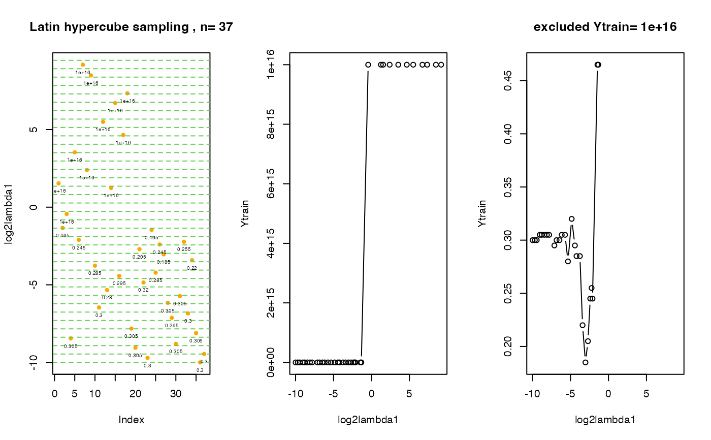
print(paste("minimal 5-fold cv error:", fit$fmin, "by log2(lambda1)=", fit$xmin))
#> [1] "minimal 5-fold cv error: 0.185 by log2(lambda1)= -3.03520543316445"
print(" all lambdas with the same minimum? ")
#> [1] " all lambdas with the same minimum? "
print(fit$ points.fmin)
#> log2lambda1 f
#> 27 -3.035205 0.185
print(paste(fit$neval, "visited points"))
#> [1] "37 visited points"
print(" overview: over all visitied points in tuning parameter space
with corresponding cv errors")
#> [1] " overview: over all visitied points in tuning parameter space \n\t\t\t\twith corresponding cv errors"
print(data.frame(Xtrain=fit$Xtrain, cv.error=fit$Ytrain))
#> log2lambda1 cv.error
#> 1 1.5315485 1.00e+16
#> 2 -1.3383552 4.65e-01
#> 3 -0.4348424 1.00e+16
#> 4 -8.4531580 3.05e-01
#> 5 3.5310332 1.00e+16
#> 6 -2.1035852 2.45e-01
#> 7 9.1782694 1.00e+16
#> 8 2.3956101 1.00e+16
#> 9 8.4905937 1.00e+16
#> 10 -3.7667024 2.85e-01
#> 11 -6.4618650 3.00e-01
#> 12 5.4976793 1.00e+16
#> 13 -5.3380199 2.80e-01
#> 14 1.2415551 1.00e+16
#> 15 6.7099483 1.00e+16
#> 16 -4.4249049 2.95e-01
#> 17 4.6509131 1.00e+16
#> 18 7.3355014 1.00e+16
#> 19 -7.8173000 3.05e-01
#> 20 -9.0531639 3.05e-01
#> 21 -2.7058843 2.05e-01
#> 22 -4.8506733 3.20e-01
#> 23 -9.7038186 3.00e-01
#> 24 -1.4557824 4.65e-01
#> 25 -4.2158845 2.85e-01
#> 26 -2.4017091 2.45e-01
#> 27 -3.0352054 1.85e-01
#> 28 -6.1636759 3.05e-01
#> 29 -7.1268118 2.95e-01
#> 30 -8.8040755 3.05e-01
#> 31 -5.7266564 3.05e-01
#> 32 -2.2278129 2.55e-01
#> 33 -6.8407343 3.00e-01
#> 34 -3.4158114 2.20e-01
#> 35 -8.1115934 3.05e-01
#> 36 -9.9999979 3.00e-01
#> 37 -9.4561642 3.00e-01
# create 3 plots om one screen:
# 1st plot: distribution of initial points in tuning parameter space
# 2nd plot: visited lambda points vs. cv errors
# 3rd plot: the same as the 2nd plot, Ytrain.exclude points are excluded.
# The value cv.error = 10^16 stays for the cv error for an empty model !
.plot.EPSGO.parms (fit$Xtrain, fit$Ytrain,bound=bounds,
Ytrain.exclude=10^16, plot.name=NULL )
 # } # end of \donttest