Find the neighborhood of a set of nodes.

Find the neighborhood of a set of nodes.

Usage

# S4 method for class 'network'
geneNeighborhood(
  net,
  targets,
  nv = 0,
  order = length(net@time_pt) - 1,
  label_v = NULL,
  ini = NULL,
  frame.color = "white",
  label.hub = FALSE,
  graph = TRUE,
  names = FALSE
)

Arguments

net

a network object

targets

a vector containing the set of nodes

nv

the level of cutoff. Defaut to 0.

order

of the neighborhood. Defaut to `length(net@time_pt)-1`.

label_v

vector defining the vertex labels.

ini

using the “position” function, you can fix the position of the nodes.

frame.color

color of the frames.

label.hub

logical ; if TRUE only the hubs are labeled.

graph

plot graph of the network. Defaults to `TRUE`.

names

return names of the neighbors. Defaults to `FALSE`.

Value

The neighborhood of the targeted genes.

References

Jung, N., Bertrand, F., Bahram, S., Vallat, L., and Maumy-Bertrand, M. (2014). Cascade: a R-package to study, predict and simulate the diffusion of a signal through a temporal gene network. Bioinformatics, btt705.

Vallat, L., Kemper, C. A., Jung, N., Maumy-Bertrand, M., Bertrand, F., Meyer, N., ... & Bahram, S. (2013). Reverse-engineering the genetic circuitry of a cancer cell with predicted intervention in chronic lymphocytic leukemia. Proceedings of the National Academy of Sciences, 110(2), 459-464.

Author

Nicolas Jung, Frédéric Bertrand , Myriam Maumy-Bertrand.

Examples

data(Selection)
data(network)
#A nv value can chosen using the cutoff function
nv=.11 
EGR1<-which(match(Selection@name,"EGR1")==1)
P<-position(network,nv=nv)

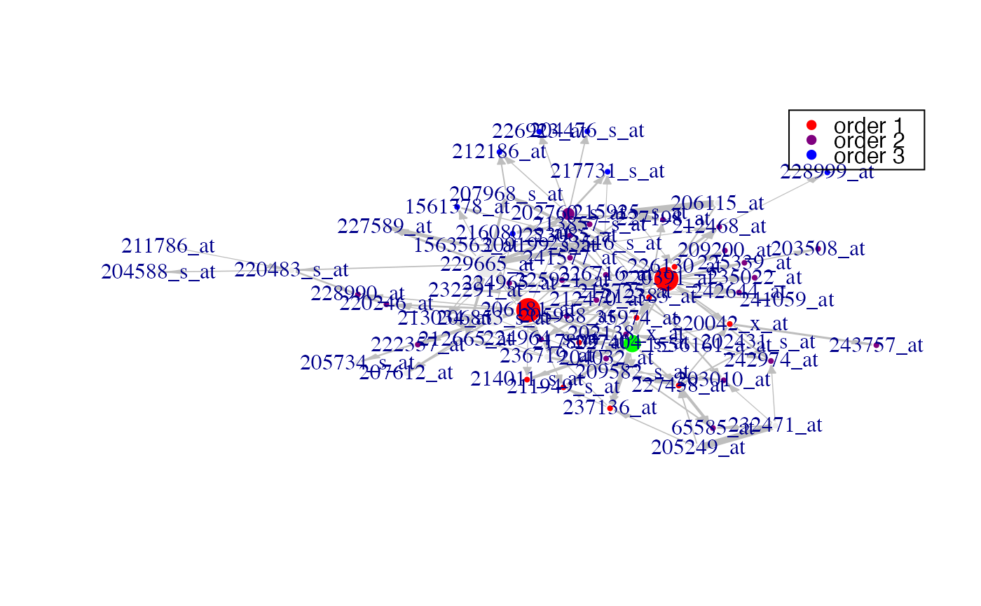
geneNeighborhood(network,targets=EGR1,nv=nv,ini=P,
label_v=network@name)

#> [[1]]
#> [[1]][[1]]
#> + 12/74 vertices, from 7a68dce:
#>  [1] 55 11 32 56 57 59 63 66 67 69 70 71
#> 
#> [[1]][[2]]
#> + 1/74 vertex, from 7a68dce:
#> [1] 68
#> 
#> 
#> [[2]]
#> [[2]][[1]]
#> + 38/74 vertices, from 7a68dce:
#>  [1] 55 11 32 56 57 59 63 66 67 69 70 71 15 16 18 20 21 22 23 24 27 30 31 42 50
#> [26] 72 40 62 48 35 38 39 19 26 37 43 45 73
#> 
#> [[2]][[2]]
#> + 1/74 vertex, from 7a68dce:
#> [1] 68
#> 
#> 
#> [[3]]
#> [[3]][[1]]
#> + 45/74 vertices, from 7a68dce:
#>  [1] 55 11 32 56 57 59 63 66 67 69 70 71 15 16 18 20 21 22 23 24 27 30 31 42 50
#> [26] 72 40 62 48 35 38 39 19 26 37 43 45 73 36 54 41 46 49 51 52
#> 
#> [[3]][[2]]
#> + 1/74 vertex, from 7a68dce:
#> [1] 68
#> 
#>