Overview
SelectBoost.quantile adapts the SelectBoost idea to
sparse quantile regression. A typical workflow is:
- fit a quantile model with
selectboost_quantile(), - inspect the selection-frequency path,
- extract a stable support with
summary()orsupport_selectboost_quantile(), - optionally tune the penalty explicitly with
tune_lambda_quantile().
The current package defaults are designed to be reasonably
conservative: screening is activated automatically in
p > n settings, tuning can use a 1-SE rule with penalty
inflation, and stable support extraction defaults to a hybrid score that
combines path stability and fitted effect size.
Simulate a correlated design
load_selectboost_quantile <- function() {
  if (requireNamespace("SelectBoost.quantile", quietly = TRUE)) {
    library(SelectBoost.quantile)
    return(invisible(TRUE))
  }

  if (!requireNamespace("pkgload", quietly = TRUE)) {
    stop(
      "SelectBoost.quantile is not installed and pkgload is unavailable.",
      call. = FALSE
    )
  }

  roots <- c(".", "..")
  roots <- roots[file.exists(file.path(roots, "DESCRIPTION"))]
  if (!length(roots)) {
    stop("Could not locate the package root for SelectBoost.quantile.", call. = FALSE)
  }

  pkgload::load_all(roots[[1]], export_all = FALSE, helpers = FALSE, quiet = TRUE)
  invisible(TRUE)
}

load_selectboost_quantile()

sim <- simulate_quantile_data(
  n = 100,
  p = 20,
  active = 1:4,
  rho = 0.7,
  correlation = "toeplitz",
  tau = 0.5,
  seed = 1
)
Fit a first model
fit <- selectboost_quantile(
  sim$x,
  sim$y,
  tau = 0.5,
  B = 6,
  step_num = 0.5,
  screen = "auto",
  tune_lambda = "cv",
  lambda_rule = "one_se",
  lambda_inflation = 1.25,
  subsamples = 4,
  sample_fraction = 0.5,
  complementary_pairs = TRUE,
  max_group_size = 10,
  seed = 1,
  verbose = FALSE
)

print(fit)
#> SelectBoost-style quantile regression sketch
#>   tau: 0.5
#>   perturbation replicates: 6
#>   c0 thresholds: 5
#>   predictors: 20
#>   grouping: group_neighbors
#>   max group size: 10
#>   screening: none
#>   stability selection: 4 draws at fraction 0.5 (complementary pairs)
#>   tuned lambda factor: 0.7789 (cv, one_se)
#>   top mean selection frequencies:
#>    x2    x1    x3    x4   x17    x5
#> 0.883 0.875 0.771 0.688 0.583 0.579
The printed object summarizes the perturbation path, tuning choice, screening rule, and the highest mean selection frequencies.
Summarize and extract stable support
smry <- summary(fit)
smry
#> Tau: 0.5
#> Stable support threshold: 0.55
#> Selection metric: hybrid
#> Variables above the threshold:
#> [1] "x2" "x1" "x3"
#> Top summary scores:
#>    x2    x1    x3    x4   x13   x17    x5   x14   x12   x10
#> 0.871 0.863 0.686 0.513 0.189 0.164 0.080 0.069 0.044 0.022

support_selectboost_quantile(fit)
#> [1] "x2" "x1" "x3"
coef(fit, threshold = 0.55)
#>   (Intercept)            x1            x2            x3            x4
#> -2.892020e-01  1.910100e+00  1.653308e+00 -9.918470e-01  6.193026e-01
#>            x5            x7           x11           x14           x17
#>  4.772659e-02 -6.892092e-12  6.177269e-11 -6.625734e-02  8.629423e-02
#>           x18           x19           x20
#>  4.285874e-12  1.149629e-11  2.044608e-11
By default, summary() and
support_selectboost_quantile() use the hybrid support
score. If you want the older frequency-only rule, use
selection_metric = "frequency".
support_selectboost_quantile(
  fit,
  threshold = 0.55,
  selection_metric = "frequency"
)
#>  [1] "x1"  "x2"  "x3"  "x4"  "x5"  "x7"  "x11" "x14" "x17" "x18" "x19" "x20"
Plot the frequency path
plot(fit)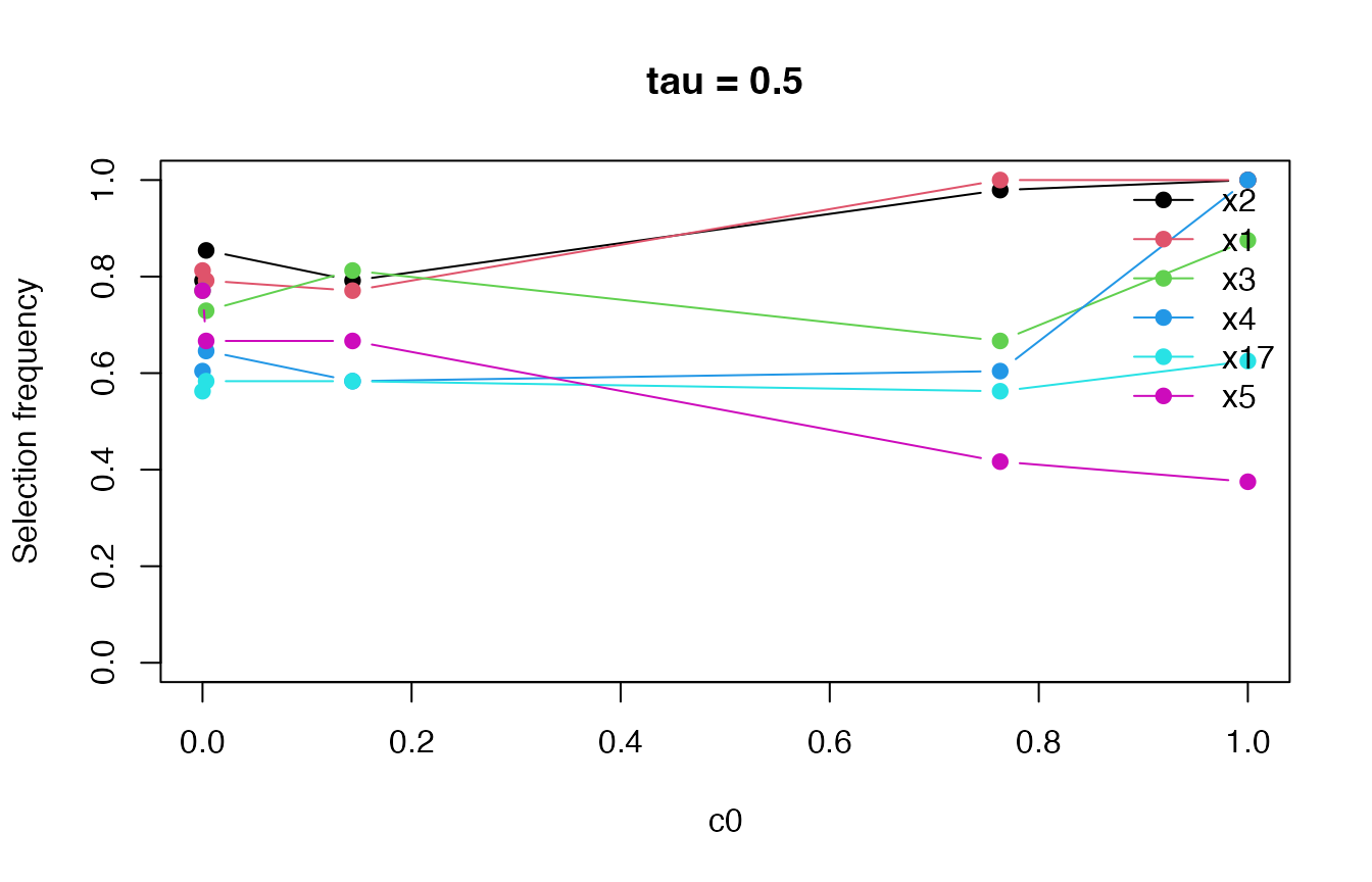
The path can help distinguish variables that remain stable under stronger perturbations from variables that are selected only when the perturbation is weak.
Formula interface and multiple quantiles
dat <- data.frame(y = sim$y, sim$x)

fit_formula <- selectboost_quantile(
  y ~ .,
  data = dat,
  tau = c(0.25, 0.5, 0.75),
  B = 4,
  step_num = 0.5,
  tune_lambda = "bic",
  seed = 2,
  verbose = FALSE
)

print(fit_formula)
#> SelectBoost-style quantile regression sketch
#>   tau: 0.25, 0.50, 0.75
#>   perturbation replicates: 4
#>   c0 thresholds: 5
#>   predictors: 20
#>   grouping: group_neighbors
#>   screening: none
#>   tuned lambda factors: 1.0000, 0.5322, 1.0000
#>  tau = 0.25: top mean selection frequencies
#>   x1   x2   x3  x20
#> 0.95 0.85 0.85 0.85
#>  tau = 0.5: top mean selection frequencies
#>  x17   x3   x4   x5
#> 0.95 0.90 0.90 0.90
#>  tau = 0.75: top mean selection frequencies
#>   x1   x3   x4  x16
#> 0.85 0.80 0.80 0.80
summary(fit_formula, tau = 0.5)
#> Tau: 0.5
#> Stable support threshold: 0.55
#> Selection metric: hybrid
#> Variables above the threshold:
#> [1] "x2" "x3" "x1"
#> Top summary scores:
#>    x2    x3    x1    x4   x17    x5   x13   x14   x12    x6
#> 0.850 0.832 0.750 0.502 0.300 0.265 0.222 0.185 0.178 0.000
Predictions can be extracted from either matrix- or formula-based fits.
predict(
  fit_formula,
  newdata = dat[1:3, -1, drop = FALSE],
  tau = 0.5
)
#>          1          2          3
#> -1.7911186  0.2847084 -2.5857687
Inspect penalty tuning directly
tuned <- tune_lambda_quantile(
  sim$x,
  sim$y,
  tau = 0.5,
  method = "cv",
  rule = "one_se",
  lambda_inflation = 1.25,
  nlambda = 6,
  folds = 3,
  repeats = 2,
  seed = 3,
  verbose = FALSE
)

print(tuned)
#> Quantile-lasso tuning
#>   tau: 0.5
#>   method: cv
#>   rule: one_se
#>   lambda inflation: 1.25
#>   folds: 3
#>   repeats: 2
#>   selected factor: 0.6866
#>   score: 0.49975
#>   standard error: 0.012345
summary(tuned)
#>   tau     factor     score           se   rule lambda_inflation selected
#> 1 0.5 1.00000000 0.5243058 0.0007634017 one_se             1.25    FALSE
#> 2 0.5 0.54928027 0.4997532 0.0123450390 one_se             1.25     TRUE
#> 3 0.5 0.30170882 0.5193880 0.0048581777 one_se             1.25    FALSE
#> 4 0.5 0.16572270 0.5402414 0.0016910207 one_se             1.25    FALSE
#> 5 0.5 0.09102821 0.5487809 0.0123171347 one_se             1.25    FALSE
#> 6 0.5 0.05000000 0.5514630 0.0199834361 one_se             1.25    FALSE
Next steps
- Use
vignette("validation-study", package = "SelectBoost.quantile")to see how the current selector compares with the lasso baselines on the shipped benchmark study. - Use
benchmark_quantile_selection()if you want to evaluate the method on a different simulation grid.