Fast Principal Component Analysis for Big Data with bigPCAcpp

Introduction

The bigPCAcpp package provides principal component analysis (PCA) routines that operate directly on bigmemory::big.matrix objects. This vignette walks through a complete analysis workflow and compares the results against the reference implementation from base R’s prcomp() to demonstrate numerical agreement.

We will use the classic iris measurement data as a small, in-memory example. Even for larger data sets stored on disk, the workflow is identical once a big.matrix descriptor has been created.

Preparing a `big.matrix`

library(bigmemory)
library(bigPCAcpp)

iris_mat <- as.matrix(iris[, 1:4])
big_iris <- as.big.matrix(iris_mat, type = "double")

Every bigPCAcpp entry point accepts the big.matrix object directly (and, for compatibility, still works with external pointers via the @address slot), allowing analyses without copying data into regular R matrices.

Running PCA with bigPCAcpp

big_pca <- pca_bigmatrix(
  xpMat = big_iris,
  center = TRUE,
  scale = TRUE,
  ncomp = 4L,
  block_size = 128L
)
str(big_pca)
#> List of 10
#>  $ sdev               : num [1:4] 1.708 0.956 0.383 0.144
#>  $ rotation           : num [1:4, 1:4] 0.521 -0.269 0.58 0.565 0.377 ...
#>  $ center             : num [1:4] 5.84 3.06 3.76 1.2
#>  $ scale              : num [1:4] 0.828 0.436 1.765 0.762
#>  $ column_sd          : num [1:4] 0.828 0.436 1.765 0.762
#>  $ eigenvalues        : num [1:4] 2.9185 0.914 0.1468 0.0207
#>  $ explained_variance : num [1:4] 0.72962 0.22851 0.03669 0.00518
#>  $ cumulative_variance: num [1:4] 0.73 0.958 0.995 1
#>  $ covariance         : num [1:4, 1:4] 1 -0.118 0.872 0.818 -0.118 ...
#>  $ nobs               : num 150
#>  - attr(*, "backend")= chr "bigmemory"
#>  - attr(*, "class")= chr [1:3] "bigpca_bigmemory" "bigpca" "list"

The returned list mirrors the structure of a prcomp object: singular values (sdev), rotation matrix (rotation), optional centering and scaling vectors, and additional diagnostics including the covariance matrix and explained variance ratios.

Comparing against `prcomp`

base_pca <- prcomp(iris_mat, center = TRUE, scale. = TRUE)

align_columns <- function(reference, target) {
  aligned <- target
  cols <- min(ncol(reference), ncol(target))
  for (j in seq_len(cols)) {
    ref <- reference[, j]
    tgt <- target[, j]
    if (sum((ref - tgt)^2) > sum((ref + tgt)^2)) {
      aligned[, j] <- -tgt
    }
  }
  aligned
}

rotation_aligned <- align_columns(base_pca$rotation, big_pca$rotation)
max_rotation_error <- max(abs(rotation_aligned - base_pca$rotation))
max_sdev_error <- max(abs(big_pca$sdev - base_pca$sdev))

big_scores <- pca_scores_bigmatrix(
  xpMat = big_iris,
  rotation = big_pca$rotation,
  center = big_pca$center,
  scale = big_pca$scale,
  block_size = 128L
)

scores_aligned <- align_columns(base_pca$x, big_scores)
max_score_error <- max(abs(scores_aligned - base_pca$x))

c(
  rotation = max_rotation_error,
  sdev = max_sdev_error,
  scores = max_score_error
)
#>     rotation         sdev       scores 
#> 3.441691e-15 1.110223e-15 7.993606e-15

The maximum absolute deviations between the base implementation and bigPCAcpp are negligible (on the order of numerical precision), showing that the out-of-core algorithm faithfully reproduces the same components and scores.

Variable relationships

The exported helpers expose common PCA diagnostics without requiring the original data matrix in memory.

loadings <- pca_variable_loadings(big_pca$rotation, big_pca$sdev)
correlations <- pca_variable_correlations(
  big_pca$rotation,
  big_pca$sdev,
  big_pca$column_sd,
  big_pca$scale
)
contributions <- pca_variable_contributions(loadings)

head(loadings)
#>            [,1]       [,2]        [,3]        [,4]
#> [1,]  0.8901688 0.36082989  0.27565767 -0.03760602
#> [2,] -0.4601427 0.88271627 -0.09361987  0.01777631
#> [3,]  0.9915552 0.02341519 -0.05444699  0.11534978
#> [4,]  0.9649790 0.06399985 -0.24298265 -0.07535950
head(correlations)
#>            [,1]       [,2]        [,3]        [,4]
#> [1,]  0.8901688 0.36082989  0.27565767 -0.03760602
#> [2,] -0.4601427 0.88271627 -0.09361987  0.01777631
#> [3,]  0.9915552 0.02341519 -0.05444699  0.11534978
#> [4,]  0.9649790 0.06399985 -0.24298265 -0.07535950
head(contributions)
#>            [,1]         [,2]       [,3]       [,4]
#> [1,] 0.27150969 0.1424440565 0.51777574 0.06827052
#> [2,] 0.07254804 0.8524748749 0.05972245 0.01525463
#> [3,] 0.33687936 0.0005998389 0.02019990 0.64232089
#> [4,] 0.31906291 0.0044812296 0.40230191 0.27415396
range(correlations)
#> [1] -0.4601427  0.9915552

Loadings match the scaled rotation matrix, correlations honour whether the PCA was computed on standardised variables and remain bounded between -1 and 1, and contributions report the relative importance of each variable within a component.

Visualising PCA results

The companion plotting helpers make it straightforward to inspect the components returned by bigPCAcpp.

pca_plot_scree(big_pca)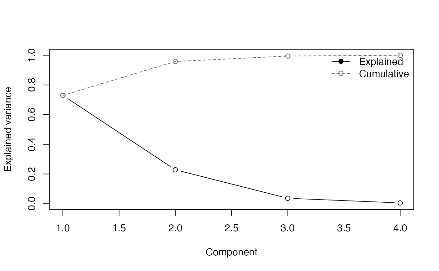

Scree plot of variance explained by each component.

The scree plot summarises how much variance each component explains and makes it easy to identify natural cutoffs.

pca_plot_scores(
  big_iris,
  rotation = big_pca$rotation,
  center = big_pca$center,
  scale = big_pca$scale,
  max_points = nrow(big_iris),
  sample = "head"
)

Scores for the first two principal components.

Score plots provide a quick way to compare sample relationships using the requested principal components without materialising the full score matrix.

pca_plot_correlation_circle(
  correlations,
  components = c(1L, 2L)
)

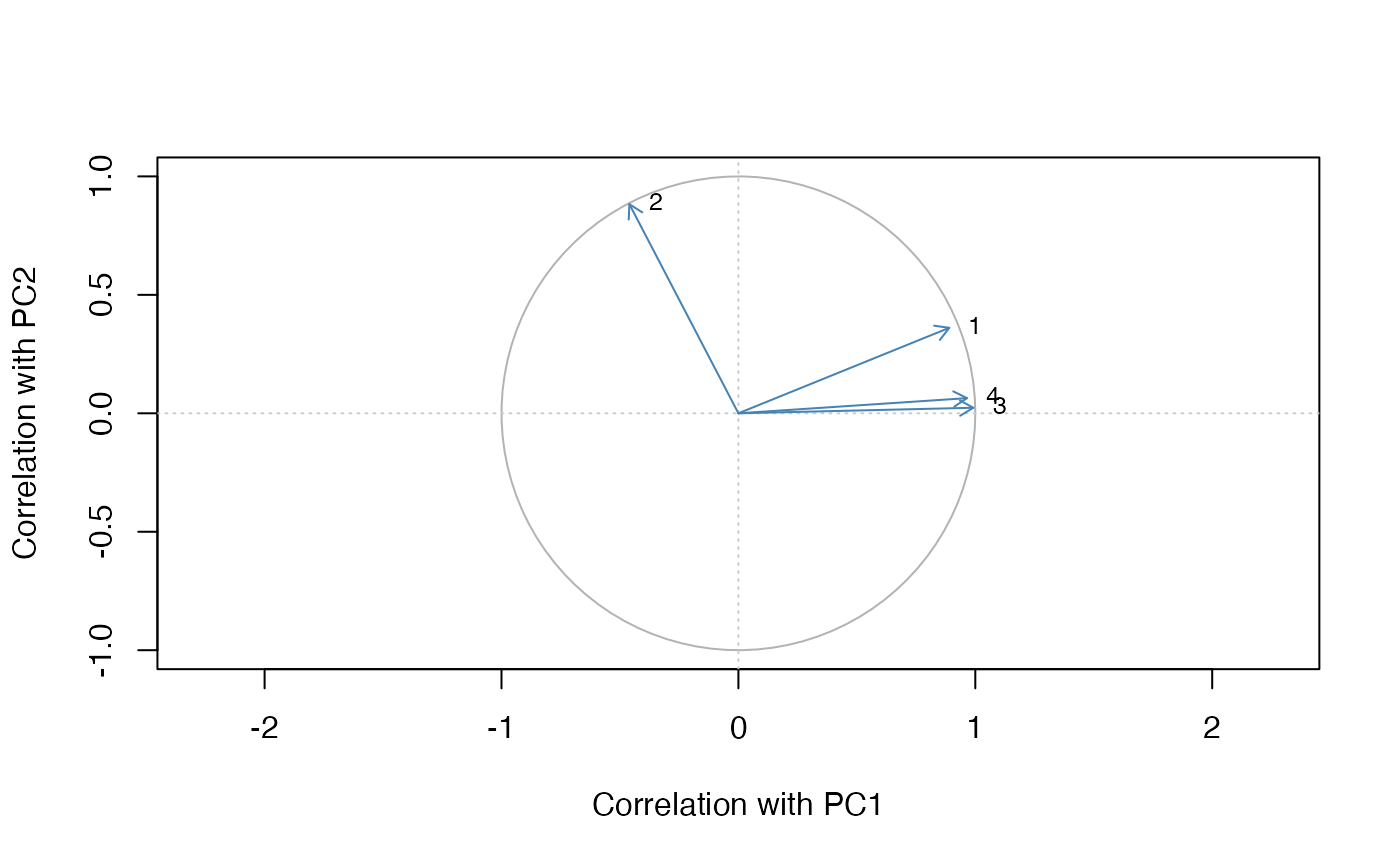
Correlation circle highlighting how variables align with the first two components.

Correlation circles visualise how each variable aligns with the chosen components, making it easy to spot groups of features that contribute in a similar direction.

pca_plot_biplot(
  big_scores,
  loadings,
  components = c(1L, 2L)
)

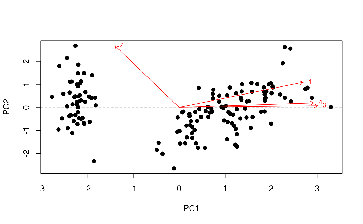
Biplot combining sample scores and variable loadings.

The biplot overlays sample scores with the variable loadings, providing a joint view of how observations cluster along the selected components and which features drive those separations.

Singular value decomposition helpers

The package also exposes building blocks for singular value decomposition (SVD) that operate directly on big.matrix instances, which can be useful for custom pipelines that only need the singular vectors or values.

svd_res <- svd_bigmatrix(big_iris, nu = 2L, nv = 2L, block_size = 128L)
svd_res$d
#> [1] 95.959914 17.761034  3.460931  1.884826

The svd_bigmatrix() helper mirrors base R’s svd() but streams data in manageable blocks, making it practical for large file-backed matrices.

Robust PCA and SVD

When data contain outliers, the robust variants supplied by bigPCAcpp help stabilise the recovered components by down-weighting leverage points.

robust_pca <- pca_robust(iris_mat, ncomp = 4L)
robust_pca$sdev
#> [1] 1.9153872 0.5075338 0.3074052 0.2357631
robust_pca$robust_weights[1:10]
#>  [1] 0.02469728 0.07676234 0.43335242 0.67140174 0.67743015 0.74308617
#>  [7] 0.65577512 0.74857591 0.79772190 0.68421285

The robust PCA interface accepts regular dense matrices, computes robust estimates of location and scale, and returns component scores along with the per-row weights and iteration counts used by the re-weighted SVD.

The underlying solver is also exposed directly for bespoke workflows that only need a robust singular value decomposition.

robust_svd <- svd_robust(iris_mat, ncomp = 3L)
robust_svd$d
#> [1] 85.31120 16.25951  3.14779
robust_svd$weights[1:10]
#>  [1] 1 1 1 1 1 1 1 1 1 1

The robust SVD returns singular values, left singular vectors, and the weights assigned to each observation, which can be combined with classical SVD results to assess the influence of individual rows.

Next steps for larger data

For on-disk matrices created with filebacked.big.matrix(), pass the descriptor pointer to pca_bigmatrix() and the algorithm will stream data in blocks, keeping memory usage bounded. Component scores can likewise be generated in batches using pca_scores_stream_bigmatrix().

library(bigmemory)
library(bigPCAcpp)

path <- tempfile(fileext = ".bin")
desc <- paste0(path, ".desc")

bm <- filebacked.big.matrix(
  nrow = nrow(iris_mat),
  ncol = ncol(iris_mat),
  type = "double",
  backingfile = basename(path),
  backingpath = dirname(path),
  descriptorfile = basename(desc)
)

bm[,] <- iris_mat

pca <- pca_bigmatrix(bm, center = TRUE, scale = TRUE, ncomp = 4)
scores <- filebacked.big.matrix(
  nrow = nrow(bm),
  ncol = ncol(pca$rotation),
  type = "double",
  backingfile = "scores.bin",
  backingpath = dirname(path),
  descriptorfile = "scores.desc"
)

pca_scores_stream_bigmatrix(
  bm,
  scores,
  pca$rotation,
  center = pca$center,
  scale = pca$scale
)
#> <pointer: 0x1507a2210>

Once the scores are stored on disk, they can be sampled and plotted just like the in-memory workflow:

pca_plot_scores(
  bm,
  rotation = pca$rotation,
  center = pca$center,
  scale = pca$scale,
  components = c(1L, 2L),
  max_points = nrow(bm),
  sample = "head"
)

Scores streamed from a file-backed big.matrix.

library(bigmemory)
library(bigPCAcpp)

path <- tempfile(fileext = ".bin")
desc <- paste0(path, ".desc")

bm <- filebacked.big.matrix(
  nrow = 5000,
  ncol = 50,
  type = "double",
  backingfile = basename(path),
  backingpath = dirname(path),
  descriptorfile = basename(desc)
)

pca <- pca_bigmatrix(bm, center = TRUE, scale = TRUE, ncomp = 5)
scores <- filebacked.big.matrix(
  nrow = nrow(bm),
  ncol = ncol(pca$rotation),
  type = "double",
  backingfile = "scores.bin",
  backingpath = dirname(path),
  descriptorfile = "scores.desc"
)

pca_scores_stream_bigmatrix(
  bm,
  scores,
  pca$rotation,
  center = pca$center,
  scale = pca$scale
)

With these building blocks, bigPCAcpp enables analyses that match the accuracy of in-memory PCA workflows while scaling to data sets that exceed RAM.

Frédéric Bertrand