Renderer Showcase Examples

Showcase Lens

This vignette assembles several scenarios meant to answer the kind of question a package user is likely to ask:

• Does the package support visually compelling, research-relevant examples?
• Can it express both generative-machine-learning and scientific-visualization workflows through a grammar familiar to R users?
• Is the current rendering surface broad enough to support a larger WebGL workflow?

The current package renders dense 2D points and lines in WebGL. The examples below stay within that supported subset on purpose.

The vignette uses the standard preset to keep article build time and page weight reasonable. The standalone gallery exporter uses detail = "high_detail" by default.

The examples also use the current shader surface deliberately:

• density_splat for dense point fields
• trajectory_age for line and path bundles
• hover inspection in addition to pan and zoom

Example 1: Latent-Space Population Structure

Why this example matters. This is the dense embedding case. It demonstrates whether ggWebGL can display cluster cores and transitional bridges in a way that feels closer to an interactive graphics system than to a static statistical scatterplot.

What to inspect. The transitional bridge should read as a continuous structure rather than as noise between clusters.

Rendering mode. This example uses shader = "density_splat" to make dense regions accumulate rather than read as a uniform cloud of isolated marks.

showcase_examples$latent_cloud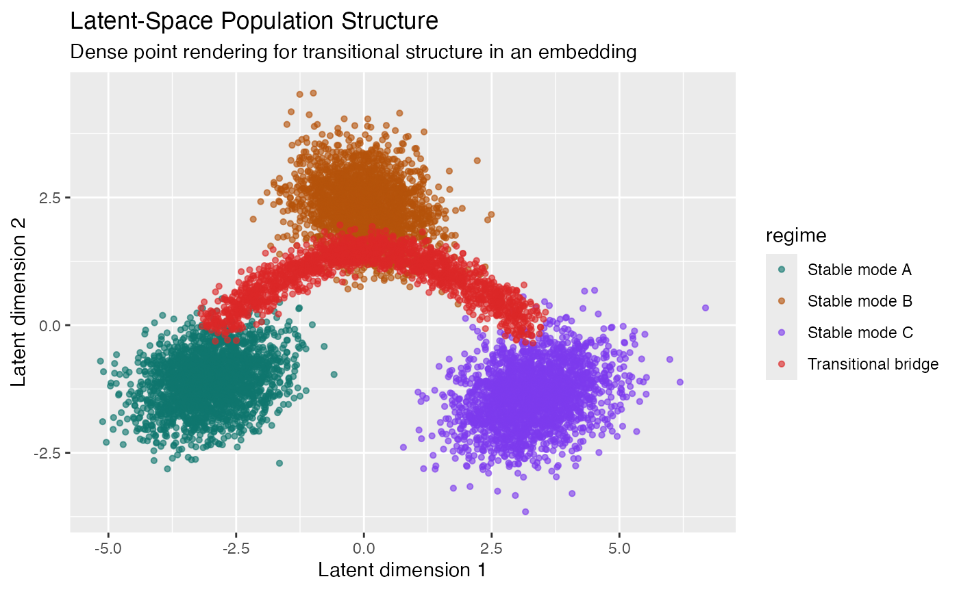

ggplot_webgl(showcase_examples$latent_cloud+theme_webgl(shader = "default", height = 630))

ggplot_webgl(showcase_examples$latent_cloud, height = 630)

Example 2: Diffusion-Style Denoising Trajectories

Why this example matters. This is the generative-ML example. It shows many simultaneous trajectories collapsing toward a small set of modes, which is the kind of dynamic structure a package user might expect from an interactive renderer demonstration.

What to inspect. Look for smooth bundles, endpoint concentration, and clear distinction between target modes.

Rendering mode. This example uses shader = "trajectory_age" so later steps are visually emphasized along each denoising path.

showcase_examples$diffusion_paths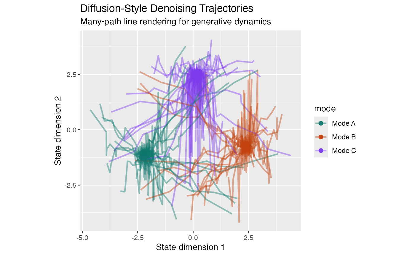

ggplot_webgl(showcase_examples$diffusion_paths+theme_webgl(shader = "default", height = 630), height = 630)

ggplot_webgl(showcase_examples$diffusion_paths, height = 630)

Example 3: Nonlinear Phase Portrait

Why this example matters. This positions ggWebGL as a scientific visualization tool rather than only as an exploratory embedding viewer. The value proposition here is that many dynamical trajectories can remain legible in an interactive browser-native plot.

What to inspect. The repeated loops and eventual convergence patterns should be visible without resorting to raster precomputation.

Rendering mode. This example also uses shader = "trajectory_age" so the flow direction remains legible in dense orbit bundles.

showcase_examples$phase_portrait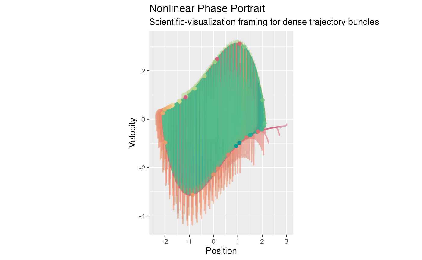

ggplot_webgl(showcase_examples$phase_portrait+theme_webgl(shader = "default"), height = 630)

ggplot_webgl(showcase_examples$phase_portrait, height = 630)

Example 4: Optimization Paths on a Surrogate Loss Landscape

Why this example matters. This is a mixed-layer example. Dense points provide a surrogate landscape while line layers show optimizer paths. It is useful because it demonstrates composition, not only raw primitive throughput.

What to inspect. The background field provides context; the traces show method-specific descent behaviour and final convergence points.

Rendering mode. This example uses shader = "density_splat" for the dense point field while leaving the optimizer traces crisp and readable.

showcase_examples$loss_landscape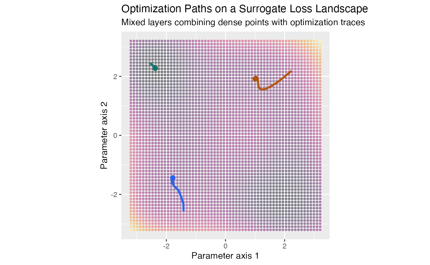

ggplot_webgl(showcase_examples$loss_landscape+theme_webgl(shader = "default"), height = 630)

ggplot_webgl(showcase_examples$loss_landscape, height = 630)

ggplot_webgl(showcase_examples$loss_landscape+theme_webgl(shader = "trajectory_age"), height = 630)

ggplot_webgl(showcase_examples$loss_landscape+theme_webgl(shader = "trajectory_age_glow"), height = 630)

Shiny Demo

The same scenarios are available in an interactive showcase Shiny app:

source(system.file("examples", "shiny", "showcase-demo.R", package = "ggWebGL"))

The standalone gallery export uses the denser preset:

source(system.file("examples", "htmlwidget", "renderer-showcase-gallery.R", package = "ggWebGL"))
export_renderer_showcase_gallery(detail = "high_detail")

This app pairs the WebGL widget with a ggplot2 reference panel so a package user can judge how much of the analytical structure already survives the current translation path.