User-friendly methods for sb_beta() results

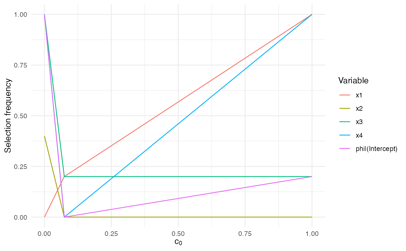
These S3 helpers make it easier to inspect and visualise the correlation-threshold grid returned by sb_beta(). They surface the stored attributes, reshape the selection frequencies into tidy summaries, and produce quick ggplot2 visualisations for interactive use.

Usage

# S3 method for class 'sb_beta'
print(x, digits = 3, ...)

# S3 method for class 'sb_beta'
summary(object, ...)

# S3 method for class 'summary.sb_beta'
print(x, digits = 3, n = 10, ...)

autoplot.sb_beta(object, variables = NULL, ...)

Arguments

x, object

An object of class sb_beta.

digits

Number of decimal places to display when printing.

...

Additional arguments passed on to lower-level methods.

n

Number of rows to show from the summary table when printing.

variables

Optional character vector of variables to retain in the plotted output.

Value

summary.sb_beta() returns an object of class summary.sb_beta containing a tidy data frame of selection frequencies. The plotting and printing methods are invoked for their side effects and return the input object invisibly.

Examples

set.seed(42)
sim <- simulation_DATA.beta(n = 50, p = 4, s = 2)
fit <- sb_beta(sim$X, sim$Y, B = 5, step.num = 0.5)
print(fit)
#> SelectBoost beta selection frequencies
#> Selector: betareg_step_aic
#> Resamples per threshold: 5
#> Interval mode: none
#> c0 grid: 1.000, 0.074, 0.000
#> Inner thresholds: 0.074
#>             x1  x2  x3  x4 phi|(Intercept)
#> c0 = 1.000 1.0 1.0 0.0 0.0               1
#> c0 = 0.074 0.0 0.2 0.2 0.0               1
#> c0 = 0.000 0.2 0.2 0.0 0.4               1
#> attr(,"c0.seq")
#> [1] 1.00000000 0.07429122 0.00000000
#> attr(,"steps.seq")
#> [1] 0.07429122
#> attr(,"B")
#> [1] 5
#> attr(,"selector")
#> [1] "betareg_step_aic"
#> attr(,"resample_diagnostics")
#> attr(,"resample_diagnostics")$`c0 = 1.000`
#> [1] group                   size                    regenerated            
#> [4] cached                  mean_abs_corr_orig      mean_abs_corr_surrogate
#> [7] mean_abs_corr_cross    
#> <0 rows> (or 0-length row.names)
#> 
#> attr(,"resample_diagnostics")$`c0 = 0.074`
#>         group size regenerated cached mean_abs_corr_orig
#> 1 x1,x2,x3,x4    4           5  FALSE         0.09585409
#> 2    x1,x2,x4    3           5  FALSE         0.14389949
#> 3       x1,x3    2           5  FALSE         0.10433716
#>   mean_abs_corr_surrogate mean_abs_corr_cross
#> 1              0.14830127          0.13174777
#> 2              0.13704850          0.10256011
#> 3              0.08700178          0.08715174
#> 
#> attr(,"resample_diagnostics")$`c0 = 0.000`
#>         group size regenerated cached mean_abs_corr_orig
#> 1 x1,x2,x3,x4    4           0   TRUE         0.09585409
#>   mean_abs_corr_surrogate mean_abs_corr_cross
#> 1               0.1483013           0.1317478
#> 
#> attr(,"interval")
#> [1] "none"
summary(fit)
#> SelectBoost beta summary
#> Selector: betareg_step_aic
#> Resamples per threshold: 5
#> Interval mode: none
#> c0 grid: 1.000, 0.074, 0.000
#> Inner thresholds: 0.074
#> Top rows:
#>        c0        variable frequency
#> 1  1.0000              x1       1.0
#> 2  1.0000              x2       0.0
#> 3  1.0000              x3       0.2
#> 4  1.0000              x4       1.0
#> 5  1.0000 phi|(Intercept)       0.2
#> 6  0.0743              x1       0.2
#> 7  0.0743              x2       0.0
#> 8  0.0743              x3       0.2
#> 9  0.0743              x4       0.0
#> 10 0.0743 phi|(Intercept)       0.0
if (requireNamespace("ggplot2", quietly = TRUE)) {
  autoplot.sb_beta(fit)
}