Simulating interval Beta data
Frédéric Bertrand
Cedric, Cnam, Parisfrederic.bertrand@lecnam.net
2025-11-04
Source:vignettes/simulate-interval-beta.Rmd
simulate-interval-beta.RmdOverview
The simulation_DATA.beta() helper produces
beta-regression design matrices paired with either fully observed
responses or interval-censored outcomes. This vignette illustrates a
typical workflow for drawing a single data set with structured
correlation and custom missingness behaviour that mimics practical
survey settings.
We simulate 300 observations with 10 candidate predictors. Four
predictors are truly associated with the response through coefficients
specified in beta_size. Correlation among predictors
follows an AR(1) structure governed by rho, which
conveniently induces near-multicollinearity while remaining
positive-definite.
sim <- simulation_DATA.beta(
  n = 300, p = 10, s = 4, beta_size = c(1.0, -0.8, 0.6, -0.5),
  corr = "ar1", rho = 0.25,
  mechanism = "mixed", mix_prob = 0.5,
  delta = function(mu, X) 0.03 + 0.02 * abs(mu - 0.5),
  alpha = function(mu, X) 0.1 + 0.05 * (mu < 0.3),
  na_rate = 0.1, na_side = "random"
)
Interval-generation parameters
The delta and alpha callbacks control how
often the simulated outcome is converted to an interval and how wide
that interval is:
-
delta(mu, X)encodes the expected half-width of the interval around the latent mean responsemu. Here we allow wider intervals when the mean is far from 0.5, highlighting heteroskedastic behaviour. -
alpha(mu, X)represents an observation-specific inflation probability. When the latent mean is below 0.3, the function returns larger values, creating more lower-bound censoring for smallmu.
With mechanism = "mixed" and
mix_prob = 0.5, half of the affected observations receive
two-sided intervals, whereas the remainder experience one-sided
censoring driven by na_side = "random".
Inspecting the simulated outcomes
The output contains the design matrix X, the fully
observed latent response Y, and the interval bounds
Y_low/Y_high. The following summaries check
the distribution of the latent response and the frequency of
interval-censoring.
summary(sim$Y)
#>      Min.   1st Qu.    Median      Mean   3rd Qu.      Max.
#> 0.0000517 0.2753408 0.5128178 0.4911643 0.6876537 0.9995677
mean(is.na(sim$Y_low) | is.na(sim$Y_high))
#> [1] 0.1
To better understand the resulting intervals we can look at a small
excerpt of the censored rows. Observations with NA on one
side correspond to one-sided censoring events.
Visualising interval widths
The difference between Y_high and Y_low
conveys how much uncertainty each interval carries. When an observation
is fully observed the bounds coincide with Y, leading to a
zero width. The histogram below demonstrates that, even with a modest
base width of 0.03, the adaptive component in delta()
creates a long right tail as the mean moves away from the centre of the
unit interval.
interval_width <- sim$Y_high - sim$Y_low
hist(interval_width, breaks = 30, col = "#0A6AA6", border = "white",
     main = "Distribution of simulated interval widths",
     xlab = "Y_high - Y_low")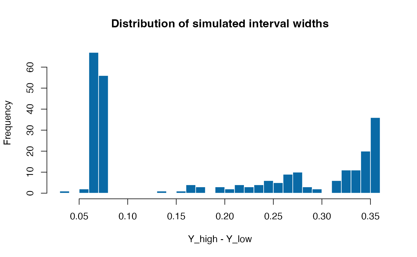
These simulated objects can be passed directly to the modelling
routines in SelectBoost.beta. The following sections
outline how to turn the generated intervals into pseudo-observations for
classical selectors, how to obtain stable frequencies with the
interval-aware fastboost routine, and how to visualise the results side
by side.
Point-response selectors on pseudo-observations
When only interval bounds are observed, a quick way to obtain a point response is to impute either the midpoint or the available bound in case of one-sided censoring. The helper below keeps the midpoint when both bounds are present and falls back to the observed edge otherwise.
pseudo_y <- ifelse(
  is.na(sim$Y_low) | is.na(sim$Y_high),
  ifelse(is.na(sim$Y_low), sim$Y_high, sim$Y_low),
  0.5 * (sim$Y_low + sim$Y_high)
)
With this pseudo-response in hand, we can deploy the full suite of
selectors shipped with the package. The
compare_selectors_single() wrapper runs the stepwise
AIC/BIC/AICc procedures, the GAMLSS-based LASSO and the
IRLS/glmnet approach in one call. Setting
include_enet = FALSE ensures the example remains
lightweight even when the optional gamlss.lasso extension
is not installed.
single <- compare_selectors_single(sim$X, pseudo_y, include_enet = FALSE)
head(single$table)
#>    selector variable       coef selected
#> x1      AIC       x1  0.9204344     TRUE
#> x2      AIC       x2 -0.7552439     TRUE
#> x3      AIC       x3  0.5566513     TRUE
#> x4      AIC       x4 -0.4996924     TRUE
#> x5      AIC       x5  0.0000000    FALSE
#> x6      AIC       x6  0.0000000    FALSE
The helper returns a list with two elements.
single$coefs stores one coefficient vector per selector
(intercept followed by the original column names), while
single$table provides a tidy summary with the
selector, variable, coef, and
selected columns. Column names are briefly shortened
internally to guarantee syntactic validity for all selectors, then
mapped back to their original labels in the returned objects.
The bootstrap helper compare_selectors_bootstrap()
repeats this exercise over resampled datasets, providing empirical
selection frequencies for each method.
freq <- compare_selectors_bootstrap(
  sim$X, pseudo_y, B = 15, include_enet = FALSE, seed = 321
)
head(freq)
#>    selector variable       freq n_success n_fail
#> x1      AIC       x1 1.00000000        15      0
#> x2      AIC       x2 1.00000000        15      0
#> x3      AIC       x3 1.00000000        15      0
#> x4      AIC       x4 1.00000000        15      0
#> x5      AIC       x5 0.26666667        15      0
#> x6      AIC       x6 0.06666667        15      0
The freq column reports the share of bootstrap
replicates in which the variable was selected. Higher values indicate
stronger evidence across resamples and help prioritise predictors for
follow-up modelling.
Merging both outputs with compare_table() gives a
compact summary containing the per-run coefficients and the associated
bootstrap frequencies.
summary_tab <- compare_table(single$table, freq)
head(summary_tab)
#>   selector variable       coef selected      freq n_success n_fail
#> 1      AIC       x1  0.9204344     TRUE 1.0000000        15      0
#> 2      AIC      x10  0.0000000    FALSE 0.2000000        15      0
#> 3      AIC       x2 -0.7552439     TRUE 1.0000000        15      0
#> 4      AIC       x3  0.5566513     TRUE 1.0000000        15      0
#> 5      AIC       x4 -0.4996924     TRUE 1.0000000        15      0
#> 6      AIC       x5  0.0000000    FALSE 0.2666667        15      0
Visual comparisons
The package offers quick visualisation helpers that default to base
graphics but automatically use ggplot2 when it is
available. The coefficient heatmap highlights which variables are
selected and their estimated effect sizes across selectors.
plot_compare_coeff(single$table)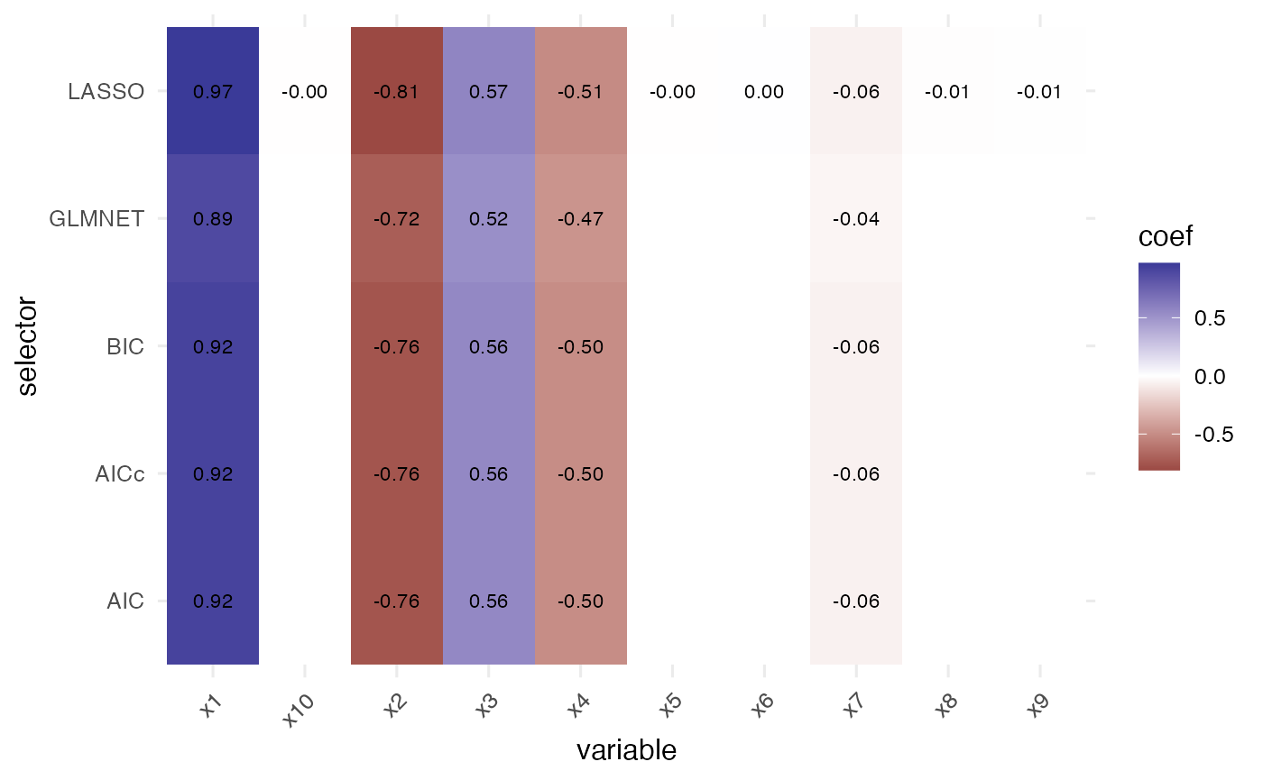
Selection frequencies from the bootstrap stage can be plotted in the same manner, providing a stability-oriented counterpart to the coefficient map.
plot_compare_freq(freq)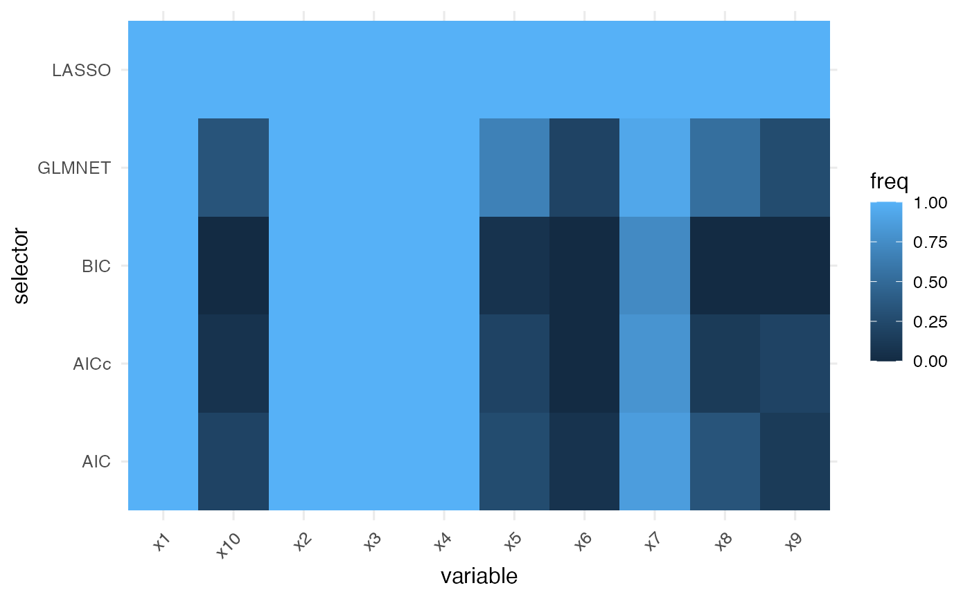
Combining both outputs with compare_table() retains the
bootstrap frequencies next to the single-run coefficients for easy
inspection.
Interval stability selection with
fastboost_interval
Instead of reducing intervals to single values, the
fastboost_interval() routine repeatedly samples
pseudo-responses inside each interval before running the chosen
selector. The resulting selection frequencies account for the
uncertainty carried by the censored observations.
fb <- fastboost_interval(
  sim$X, sim$Y_low, sim$Y_high,
  func = function(X, y) betareg_glmnet(X, y, choose = "bic", prestandardize = TRUE),
  B = 30, seed = 99
)
sort(fb$freq, decreasing = TRUE)[1:5]
#>        x1        x2        x3        x4        x8
#> 1.0000000 1.0000000 1.0000000 1.0000000 0.7333333
These additions demonstrate how the simulation engine, the collection of selectors, and the fast interval booster interact in a cohesive workflow for interval-valued beta regression problems.
Interval SelectBoost with sb_beta_interval
When you want to run the full SelectBoost workflow on interval data,
the sb_beta_interval() wrapper calls sb_beta()
with the appropriate interval sampling mode under the hood. It keeps the
same output structure as other sb_beta() runs, including
the stability matrix and diagnostic attributes.
comp_id <- complete.cases(sim$Y_low) & complete.cases(sim$Y_high)
sb_interval <- sb_beta_interval(
sim$X[comp_id, ],
Y_low = sim$Y_low[comp_id],
Y_high = sim$Y_high[comp_id],
B = 30,
step.num = 0.4,
sample = "uniform"
)
attr(sb_interval, "interval")
#> [1] "uniform"
head(sb_interval)
#> x1 x2 x3 x4 x5 x6
#> c0 = 1.000 1.00000000 1.00000000 1.0000000 1.0000000 0.1666667 0.1333333
#> c0 = 0.138 0.16666667 0.10000000 0.1000000 0.1666667 0.1666667 0.1000000
#> c0 = 0.055 0.06666667 0.23333333 0.2666667 0.2666667 0.2333333 0.1333333
#> c0 = 0.000 0.13333333 0.06666667 0.2000000 0.1000000 0.1666667 0.1000000
#> x7 x8 x9 x10 phi|(Intercept)
#> c0 = 1.000 0.5666667 0.3333333 0.00000000 0.23333333 1
#> c0 = 0.138 0.2000000 0.1333333 0.23333333 0.03333333 1
#> c0 = 0.055 0.1333333 0.1333333 0.13333333 0.16666667 1
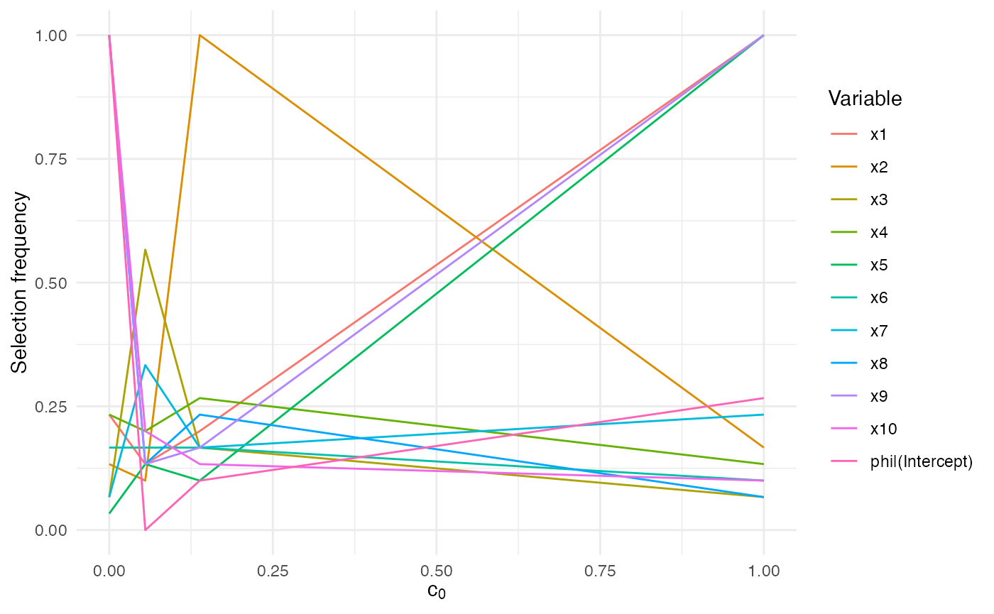
#> c0 = 0.000 0.1666667 0.2000000 0.06666667 0.06666667 1Pair this output with the plotting methods
(autoplot.sb_beta(), summary()) to inspect the
stability matrix produced under interval resampling.
summary(sb_interval)
#> SelectBoost beta summary
#> Selector: betareg_step_aic
#> Resamples per threshold: 30
#> Interval mode: uniform
#> c0 grid: 1.000, 0.138, 0.055, 0.000
#> Inner thresholds: 0.138, 0.055
#> Top rows:
#>    c0 variable frequency
#> 1   1       x1    1.0000
#> 2   1       x2    0.1667
#> 3   1       x3    0.0667
#> 4   1       x4    0.1333
#> 5   1       x5    1.0000
#> 6   1       x6    0.1000
#> 7   1       x7    0.2333
#> 8   1       x8    0.0667
#> 9   1       x9    1.0000
#> 10  1      x10    0.1000
autoplot.sb_beta(sb_interval)