Getting started with SelectBoost.beta
SelectBoost.beta authors
Cedric, Cnam, Parisfrederic.bertrand@lecnam.net
2025-11-04
Source:vignettes/selectboost-cran.Rmd
selectboost-cran.RmdIntroduction
This vignette provides a CRAN-friendly tour of the SelectBoost.beta
workflow. It simulates a reproducible beta-regression data set, runs the
high-level sb_beta() driver, and shows how to interpret the
stability matrix returned by the algorithm. All code is self-contained
and executes quickly under the default knitr settings.
Simulated data
We use the built-in simulation_DATA.beta() helper to
generate a correlated design with three truly associated predictors. The
response lives in (0, 1) and is already compatible with the
beta-regression selectors.
sim <- simulation_DATA.beta(n = 120, p = 6, s = 3, rho = 0.35,
  beta_size = c(1.1, -0.9, 0.7))
str(sim$X)
#>  num [1:120, 1:6] 0.982 0.469 -0.108 -0.213 1.158 ...
#>  - attr(*, "dimnames")=List of 2
#>   ..$ : NULL
#>   ..$ : chr [1:6] "x1" "x2" "x3" "x4" ...
summary(sim$Y)
#>      Min.   1st Qu.    Median      Mean   3rd Qu.      Max.
#> 6.685e-05 1.907e-01 5.068e-01 4.763e-01 7.551e-01 9.862e-01
Running sb_beta()
The sb_beta() wrapper orchestrates the full SelectBoost
loop: it normalises the design matrix, groups correlated predictors,
regenerates surrogate designs, and records selection frequencies for
each threshold.
sb <- sb_beta(sim$X, sim$Y, B = 40, step.num = 0.4, seed = 99)
sb
#> SelectBoost beta selection frequencies
#> Selector: betareg_step_aic
#> Resamples per threshold: 40
#> Interval mode: none
#> c0 grid: 1.000, 0.124, 0.078, 0.000
#> Inner thresholds: 0.124, 0.078
#>               x1    x2    x3    x4    x5    x6 phi|(Intercept)
#> c0 = 1.000 1.000 1.000 1.000 0.000 0.000 0.000               1
#> c0 = 0.124 0.175 0.250 1.000 0.150 0.125 0.225               1
#> c0 = 0.078 0.225 0.150 0.225 0.125 0.125 0.300               1
#> c0 = 0.000 0.175 0.225 0.125 0.050 0.125 0.175               1
#> attr(,"c0.seq")
#> [1] 1.0000000 0.1244760 0.0780104 0.0000000
#> attr(,"steps.seq")
#> [1] 0.1244760 0.0780104
#> attr(,"B")
#> [1] 40
#> attr(,"selector")
#> [1] "betareg_step_aic"
#> attr(,"resample_diagnostics")
#> attr(,"resample_diagnostics")$`c0 = 1.000`
#> [1] group                   size                    regenerated
#> [4] cached                  mean_abs_corr_orig      mean_abs_corr_surrogate
#> [7] mean_abs_corr_cross
#> <0 rows> (or 0-length row.names)
#>
#> attr(,"resample_diagnostics")$`c0 = 0.124`
#>      group size regenerated cached mean_abs_corr_orig mean_abs_corr_surrogate
#> 1 x1,x4,x5    3          40  FALSE          0.1127816               0.1356965
#> 2    x2,x6    2          40  FALSE          0.1244760               0.1294831
#> 3 x1,x4,x6    3          40  FALSE          0.1396964               0.1407319
#> 4    x1,x5    2          40  FALSE          0.1401757               0.1481810
#> 5 x2,x4,x6    3          40  FALSE          0.1374098               0.1355264
#>   mean_abs_corr_cross
#> 1          0.06758135
#> 2          0.07596385
#> 3          0.07866263
#> 4          0.06583547
#> 5          0.08691954
#>
#> attr(,"resample_diagnostics")$`c0 = 0.078`
#>            group size regenerated cached mean_abs_corr_orig
#> 1 x1,x3,x4,x5,x6    5          40  FALSE         0.09727572
#> 2    x2,x3,x4,x6    4          40  FALSE         0.10188328
#> 3 x1,x2,x3,x5,x6    5          40  FALSE         0.08631999
#> 4    x1,x2,x4,x6    4          40  FALSE         0.11819411
#> 5       x1,x3,x5    3          40  FALSE         0.10711418
#> 6 x1,x2,x3,x4,x6    5          40  FALSE         0.10113912
#>   mean_abs_corr_surrogate mean_abs_corr_cross
#> 1               0.1123564          0.07043535
#> 2               0.1156346          0.07450001
#> 3               0.1108955          0.07185240
#> 4               0.1303823          0.07356340
#> 5               0.1054951          0.06943202
#> 6               0.1183650          0.07719288
#>
#> attr(,"resample_diagnostics")$`c0 = 0.000`
#>               group size regenerated cached mean_abs_corr_orig
#> 1 x1,x2,x3,x4,x5,x6    6          40  FALSE         0.09172931
#>   mean_abs_corr_surrogate mean_abs_corr_cross
#> 1               0.1091279           0.0750416
#>
#> attr(,"interval")
#> [1] "none"
The returned matrix has one row per correlation threshold. Attributes attached to the matrix document how the fit was produced:
attr(sb, "c0.seq")
#> [1] 1.0000000 0.1244760 0.0780104 0.0000000
attr(sb, "B")
#> [1] 40
attr(sb, "interval")
#> [1] "none"
Use summary() to obtain per-threshold summaries and
autoplot.sb_beta() (when ggplot2 is available)
to visualise the stability matrix.
summary(sb)
#> SelectBoost beta summary
#> Selector: betareg_step_aic
#> Resamples per threshold: 40
#> Interval mode: none
#> c0 grid: 1.000, 0.124, 0.078, 0.000
#> Inner thresholds: 0.124, 0.078
#> Top rows:
#>       c0        variable frequency
#> 1  1.000              x1     1.000
#> 2  1.000              x2     0.175
#> 3  1.000              x3     0.225
#> 4  1.000              x4     0.175
#> 5  1.000              x5     1.000
#> 6  1.000              x6     0.250
#> 7  1.000 phi|(Intercept)     0.150
#> 8  0.124              x1     0.225
#> 9  0.124              x2     1.000
#> 10 0.124              x3     1.000
if (requireNamespace("ggplot2", quietly = TRUE)) {
  autoplot.sb_beta(sb)
}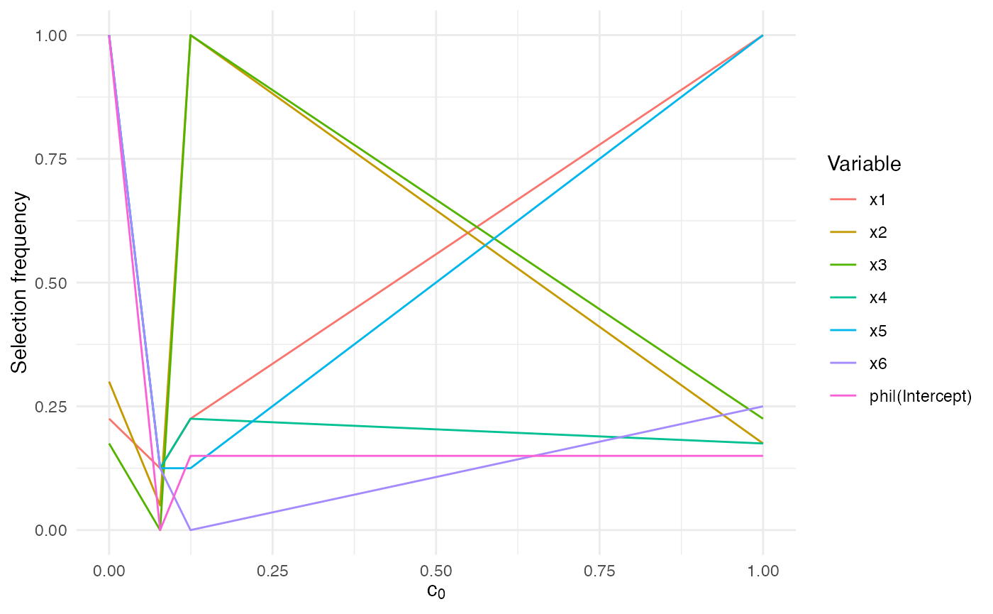
The frequency values range between 0 and 1 and report how often each
predictor received a non-zero coefficient across the correlated
replicates. High values signal stable selections. If your data contain
zeros or ones, keep squeeze = TRUE (the default) so the
algorithm applies the standard SelectBoost transformation before fitting
the selectors.
Comparing selectors
When you wish to benchmark multiple selector families, the
compare_selectors_single() helper runs them once on the
same data set and returns both raw coefficients and a tidy summary
table. Column names are briefly shortened internally to satisfy each
selector and then mapped back in the outputs.
single <- compare_selectors_single(sim$X, sim$Y, include_enet = FALSE)
head(single$table)
#>    selector variable       coef selected
#> x1      AIC       x1  1.0590158     TRUE
#> x2      AIC       x2 -0.8855152     TRUE
#> x3      AIC       x3  0.7277844     TRUE
#> x4      AIC       x4  0.0000000    FALSE
#> x5      AIC       x5  0.0000000    FALSE
#> x6      AIC       x6  0.0000000    FALSE
Bootstrap tallies add a stability perspective. The freq
column in the table below measures the proportion of resamples where the
variable was selected; values close to 1 indicate consistent
discoveries.
freq <- suppressWarnings(compare_selectors_bootstrap(sim$X, sim$Y, B = 100,
                                                     include_enet = FALSE, seed = 99))
head(freq)
#>    selector variable freq n_success n_fail
#> x1      AIC       x1 1.00       100      0
#> x2      AIC       x2 1.00       100      0
#> x3      AIC       x3 1.00       100      0
#> x4      AIC       x4 0.22       100      0
#> x5      AIC       x5 0.17       100      0
#> x6      AIC       x6 0.32       100      0
Merge both views with compare_table() and use
plot_compare_coeff() or plot_compare_freq()
for quick diagnostics.
compare_table(single$table, freq)
#>    selector variable          coef selected freq n_success n_fail
#> 1       AIC       x1  1.059016e+00     TRUE 1.00       100      0
#> 2       AIC       x2 -8.855152e-01     TRUE 1.00       100      0
#> 3       AIC       x3  7.277844e-01     TRUE 1.00       100      0
#> 4       AIC       x4  0.000000e+00    FALSE 0.22       100      0
#> 5       AIC       x5  0.000000e+00    FALSE 0.17       100      0
#> 6       AIC       x6  0.000000e+00    FALSE 0.32       100      0
#> 7      AICc       x1  1.059016e+00     TRUE 1.00       100      0
#> 8      AICc       x2 -8.855152e-01     TRUE 1.00       100      0
#> 9      AICc       x3  7.277844e-01     TRUE 1.00       100      0
#> 10     AICc       x4  0.000000e+00    FALSE 0.16       100      0
#> 11     AICc       x5  0.000000e+00    FALSE 0.13       100      0
#> 12     AICc       x6  0.000000e+00    FALSE 0.37       100      0
#> 13      BIC       x1  1.059016e+00     TRUE 1.00       100      0
#> 14      BIC       x2 -8.855152e-01     TRUE 1.00       100      0
#> 15      BIC       x3  7.277844e-01     TRUE 1.00       100      0
#> 16      BIC       x4  0.000000e+00    FALSE 0.02       100      0
#> 17      BIC       x5  0.000000e+00    FALSE 0.03       100      0
#> 18      BIC       x6  0.000000e+00    FALSE 0.13       100      0
#> 19   GLMNET       x1  9.901824e-01     TRUE 1.00       100      0
#> 20   GLMNET       x2 -8.043564e-01     TRUE 1.00       100      0
#> 21   GLMNET       x3  6.703246e-01     TRUE 1.00       100      0
#> 22   GLMNET       x4  0.000000e+00    FALSE 0.30       100      0
#> 23   GLMNET       x5  0.000000e+00    FALSE 0.41       100      0
#> 24   GLMNET       x6  0.000000e+00    FALSE 0.49       100      0
#> 25    LASSO       x1  1.088734e+00     TRUE 1.00       100      0
#> 26    LASSO       x2 -8.211508e-01     TRUE 1.00       100      0
#> 27    LASSO       x3  7.489369e-01     TRUE 1.00       100      0
#> 28    LASSO       x4  5.275007e-11     TRUE 1.00       100      0
#> 29    LASSO       x5 -1.981396e-05     TRUE 1.00       100      0
#> 30    LASSO       x6  4.151315e-02     TRUE 1.00       100      0
Interval responses
If your outcome is interval-censored, run the
sb_beta_interval() convenience wrapper. It enables the
interval sampling logic inside sb_beta() while keeping the
same output format and attributes.
y_low <- pmax(sim$Y - 0.05, 0)
y_high <- pmin(sim$Y + 0.05, 1)
interval_fit <- sb_beta_interval(sim$X, y_low, y_high, B = 30,
  sample = "uniform", seed = 321)
attr(interval_fit, "interval")
#> [1] "uniform"
The resulting stability matrix can be summarised and visualised exactly like the point-response output shown earlier. ```