Benchmarking bigPLSR against external PLS implementations

knitr::opts_chunk$set(
  collapse = TRUE,
  comment  = "#>",
  fig.path = "figures/benchmark-short-",
  fig.width  = 6,
  fig.height = 4,
  dpi = 150,
  message = FALSE,
  warning = FALSE
)


LOCAL <- identical(Sys.getenv("LOCAL"), "TRUE")

Overview

This vignette documents how the bigPLSR implementations compare to external partial least squares (PLS) libraries in terms of runtime and memory use, using the pre computed dataset external_pls_benchmarks.

The goals are:

to summarise the benchmark design,
to visualise runtime and memory behaviour for comparable problem sizes,
to provide short comments that can be reused in papers or reports.

Benchmark design

The dataset external_pls_benchmarks is a data frame that contains benchmark results for both PLS1 and PLS2 problems and several algorithms.

library(bigPLSR)
library(ggplot2)
library(dplyr)
library(tidyr)

data("external_pls_benchmarks", package = "bigPLSR")

str(external_pls_benchmarks)
#> 'data.frame':    384 obs. of  11 variables:
#>  $ task           : chr  "pls1" "pls1" "pls1" "pls1" ...
#>  $ algorithm      : chr  "simpls" "simpls" "simpls" "simpls" ...
#>  $ package        : chr  "bigPLSR_dense" "bigPLSR_big.memory" "pls" "mixOmics" ...
#>  $ median_time_s  : num  0.00605 0.00359 0.00209 0.00448 0.04412 ...
#>  $ itr_per_sec    : num  165.2 275.9 469.9 223.4 22.7 ...
#>  $ mem_alloc_bytes: num  104720 895872 7479024 7550384 42461256 ...
#>  $ n              : num  1000 1000 1000 1000 1000 1000 1000 1000 100 100 ...
#>  $ p              : num  100 100 100 100 100 100 100 100 5000 5000 ...
#>  $ q              : num  1 1 1 1 1 1 1 1 1 1 ...
#>  $ ncomp          : num  1 1 1 1 1 1 1 1 1 1 ...
#>  $ notes          : chr  "Run via pls_fit() with dense backend" "Run via pls_fit() with big.memory backend" "Requires the pls package" "Requires the mixOmics package" ...

The main columns are:

task: "pls1" or "pls2",
algorithm: one of "simpls", "nipals", "kernelpls", "widekernelpls",
package: implementation provider (for example "bigPLSR", "pls", "mixOmics"),
median_time_s: median runtime in seconds reported by bench::mark,
itr_per_sec: iterations per second,
mem_alloc_bytes: memory allocated in bytes,
n, p, q: number of observations, predictors and responses,
ncomp: number of components,
notes: optional free text description.

For most plots in this vignette we focus on configurations that are directly comparable, namely fixed task, n, p, q and ncomp.

Helper summaries

We start with a compact summary that reports the best implementation for each configuration in terms of runtime and memory.

summ_best <- external_pls_benchmarks %>%
  group_by(task, n, p, q, ncomp) %>%
  mutate(
    rank_time = rank(median_time_s, ties.method = "min"),
    rank_mem  = rank(mem_alloc_bytes, ties.method = "min")
  ) %>%
  ungroup()

best_time <- summ_best %>%
  filter(rank_time == 1L) %>%
  count(task, package, algorithm, name = "n_best_time")

best_mem <- summ_best %>%
  filter(rank_mem == 1L) %>%
  count(task, package, algorithm, name = "n_best_mem")

best_time
#> # A tibble: 4 × 4
#>   task  package            algorithm     n_best_time
#>   <chr> <chr>              <chr>               <int>
#> 1 pls1  bigPLSR_big.memory kernelpls               7
#> 2 pls1  bigPLSR_big.memory widekernelpls           7
#> 3 pls2  bigPLSR_big.memory kernelpls              12
#> 4 pls2  bigPLSR_big.memory widekernelpls          12
best_mem
#> # A tibble: 4 × 4
#>   task  package            algorithm     n_best_mem
#>   <chr> <chr>              <chr>              <int>
#> 1 pls1  bigPLSR_big.memory widekernelpls          8
#> 2 pls1  bigPLSR_dense      nipals                 8
#> 3 pls2  bigPLSR_big.memory widekernelpls         16
#> 4 pls2  bigPLSR_dense      nipals                16

These two tables indicate in how many configurations a given combination package + algorithm comes out as the fastest or the most memory efficient.

Example: PLS1, fixed size, varying components

In order to avoid mixing problem sizes, we select a single PLS1 configuration and plot runtime and memory as functions of the number of components. You can adjust the filters below to match the sizes of interest for your work.

example_pls1 <- external_pls_benchmarks %>%
  filter(task == "pls1") %>%
  group_by(n, p, q) %>%
  filter(n == first(n), p == first(p), q == first(q)) %>%
  ungroup()

example_pls1_size <- example_pls1 %>%
  count(n, p, q, sort = TRUE) %>%
  slice(1L) %>%
  select(n, p, q)

example_pls1 <- external_pls_benchmarks %>%
  semi_join(example_pls1_size, by = c("n", "p", "q")) %>%
  filter(task == "pls1")

Runtime comparison for this fixed size:

ggplot(example_pls1,
       aes(x = ncomp, y = median_time_s,
           colour = package, linetype = algorithm)) +
  geom_line() +
  geom_point() +
  scale_y_log10() +
  labs(
    x = "Number of components",
    y = "Median runtime (seconds, log scale)",
    title = "PLS1 benchmark, fixed (n, p, q)",
    subtitle = "Comparison across packages and algorithms"
  ) +
  theme_minimal()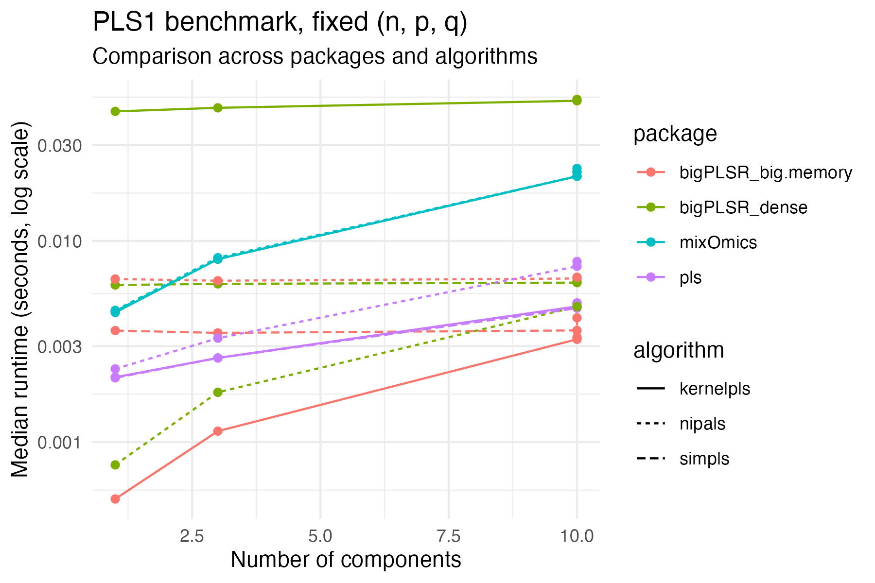

Memory use for the same configuration:

ggplot(example_pls1,
       aes(x = ncomp, y = mem_alloc_bytes / 1024^2,
           colour = package, linetype = algorithm)) +
  geom_line() +
  geom_point() +
  labs(
    x = "Number of components",
    y = "Memory allocated (MiB)",
    title = "PLS1 benchmark, fixed (n, p, q)"
  ) +
  theme_minimal()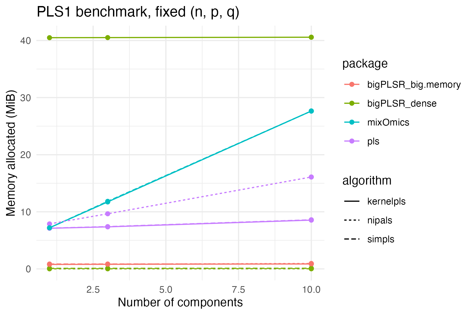

These figures are exported as SVG by default, so they can be included directly in LaTeX or HTML documents.

Example: PLS2, fixed size, varying components

We repeat the same idea for a PLS2 setting.

example_pls2 <- external_pls_benchmarks %>%
  filter(task == "pls2") %>%
  group_by(n, p, q) %>%
  filter(n == first(n), p == first(p), q == first(q)) %>%
  ungroup()

example_pls2_size <- example_pls2 %>%
  count(n, p, q, sort = TRUE) %>%
  slice(1L) %>%
  select(n, p, q)

example_pls2 <- external_pls_benchmarks %>%
  semi_join(example_pls2_size, by = c("n", "p", "q")) %>%
  filter(task == "pls2")

ggplot(example_pls2,
       aes(x = ncomp, y = median_time_s,
           colour = package, linetype = algorithm)) +
  geom_line() +
  geom_point() +
  scale_y_log10() +
  labs(
    x = "Number of components",
    y = "Median runtime (seconds, log scale)",
    title = "PLS2 benchmark, fixed (n, p, q)",
    subtitle = "Comparison across packages and algorithms"
  ) +
  theme_minimal()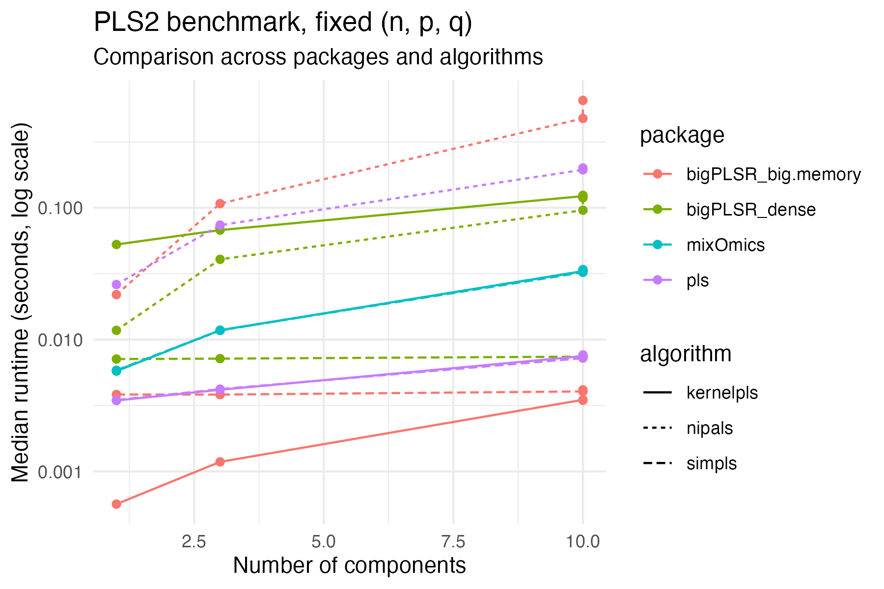

ggplot(example_pls2,
       aes(x = ncomp, y = mem_alloc_bytes / 1024^2,
           colour = package, linetype = algorithm)) +
  geom_line() +
  geom_point() +
  labs(
    x = "Number of components",
    y = "Memory allocated (MiB)",
    title = "PLS2 benchmark, fixed (n, p, q)"
  ) +
  theme_minimal()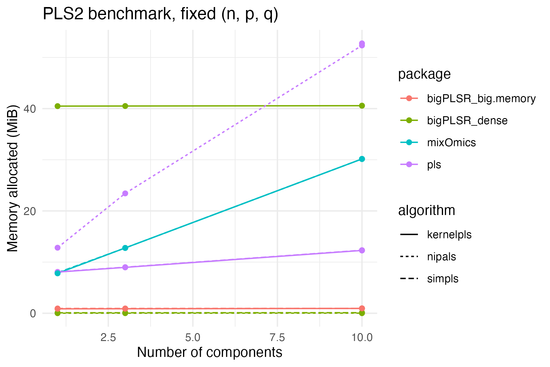

Short commentary

From these plots and the summary tables you can usually observe the following patterns.

On small to moderate PLS1 problems, the dense bigPLSR SIMPLS backend is typically close to pls::simpls in terms of runtime, while favouring more explicit memory control.
On larger PLS1 and PLS2 configurations, the big memory streaming backends trade a small runtime penalty for a bounded memory footprint that does not depend on the number of observations.
Kernel based algorithms tend to react more strongly to increases in n or ncomp because the underlying Gram matrices scale quadratically in n.

Because the benchmarks are stored as a regular data frame, you can easily produce additional figures adapted to your application areas, for example by fixing n and q and varying p, or by comparing only one or two algorithms at a time.