Bootstrap strategies for bigPLSR

Introduction

bigPLSR now provides two complementary bootstrap procedures:

(X, Y) bootstrap refits the full regression model on resampled pairs.
(X, T) bootstrap keeps the latent components of the original fit and resamples the score structure, delivering fast updates of the regression coefficients.

Both approaches expose percentile and BCa confidence intervals, numerical summaries and plotting helpers.

We rely on a small multivariate example to illustrate the workflow.

library(bigPLSR)
n <- 100; p <- 6; m <- 2
X <- matrix(rnorm(n * p), n, p)
eta1 <- X[, 1] + 0.4 * X[, 2] - 0.6 * X[, 3]
eta2 <- -0.5 * X[, 2] + 0.7 * X[, 4] + 0.5 * X[, 5]
Y <- cbind(eta1, eta2) + matrix(rnorm(n * m, sd = 0.5), n, m)

Baseline fit

fit <- pls_fit(X, Y, ncomp = 3, scores = "r")

(X, Y) bootstrap

boot_xy <- pls_bootstrap(X, Y, ncomp = 3, R = 50, type = "xy",
                         parallel = "none", return_scores = TRUE)
head(summarise_pls_bootstrap(boot_xy))
#>   variable response        mean         sd percentile_lower percentile_upper
#> 1       X1       Y1  1.12720380 0.05483111       1.03357126       1.22790239
#> 2       X2       Y1  0.31715126 0.07184301       0.16076652       0.43387511
#> 3       X3       Y1 -0.58032760 0.07402063      -0.71756064      -0.44816272
#> 4       X4       Y1  0.01629040 0.07403399      -0.13117394       0.11615478
#> 5       X5       Y1  0.03428052 0.08010332      -0.09078452       0.17987746
#> 6       X6       Y1 -0.02468821 0.05931838      -0.14013792       0.07848342
#>     bca_lower  bca_upper
#> 1  1.07662505  1.2870309
#> 2  0.11687183  0.4120490
#> 3 -0.71386459 -0.3935652
#> 4 -0.18829055  0.1576646
#> 5 -0.09981499  0.3233262
#> 6 -0.14153533  0.0540529

A quick visual inspection of the coefficient distributions:

plot_pls_bootstrap_coefficients(boot_xy, variables = colnames(X))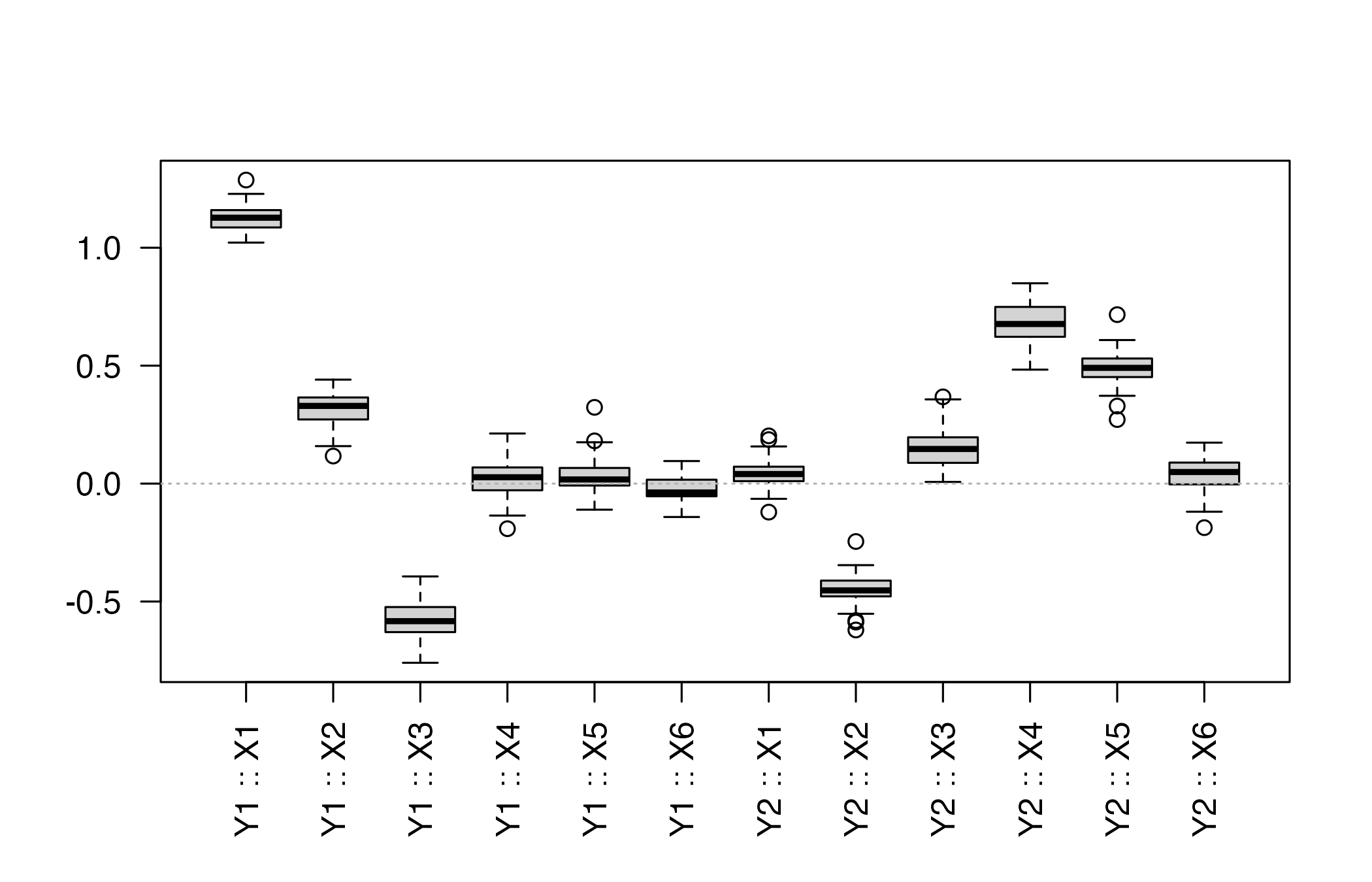

(X, T) bootstrap

The conditional bootstrap operates on the latent score representation extracted from the baseline fit.

boot_xt <- pls_bootstrap(X, Y, ncomp = 3, R = 50, type = "xt",
                         parallel = "none", return_scores = TRUE)
head(summarise_pls_bootstrap(boot_xt))
#>   variable response        mean         sd percentile_lower percentile_upper
#> 1       X1     eta1  1.14632807 0.04497402        1.0672858      1.216945852
#> 2       X2     eta1  0.31388701 0.03309151        0.2577740      0.376551867
#> 3       X3     eta1 -0.57958235 0.02422587       -0.6339318     -0.539038171
#> 4       X4     eta1  0.01363128 0.03222957       -0.0448380      0.069097207
#> 5       X5     eta1  0.01377627 0.03246635       -0.0569404      0.072171472
#> 6       X6     eta1 -0.04337170 0.02979694       -0.1021070     -0.004940322
#>     bca_lower   bca_upper
#> 1  1.06165429  1.22675518
#> 2  0.25417756  0.38356573
#> 3 -0.62915894 -0.51626603
#> 4 -0.05084027  0.07010002
#> 5 -0.03361595  0.07498808
#> 6 -0.12270539  0.02059054

plot_pls_bootstrap_coefficients(boot_xt, responses = colnames(Y))

Exploring bootstrap scores

When return_scores = TRUE, the bootstrap result stores the score matrices for each replicate. This allows for custom diagnostics such as the dispersion of the first two latent variables:

score_mats <- boot_xt$score_samples
score_means <- sapply(score_mats, function(M) colMeans(M)[1:2])
apply(score_means, 1, summary)
#>                 [,1]          [,2]
#> Min.    -0.023265400 -0.0177317599
#> 1st Qu. -0.010183238 -0.0067989105
#> Median  -0.002768175 -0.0013845304
#> Mean    -0.002329194 -0.0006864936
#> 3rd Qu.  0.004474621  0.0059661965
#> Max.     0.021550597  0.0225250130

You can feed individual score matrices into plot_pls_individuals() to overlay confidence ellipses obtained from the bootstrap draws.

Parallel execution

Both bootstrap flavours honour the parallel = "future" option. Configure your preferred plan before calling the helper:

future::plan(future::multisession, workers = 2)
boot_xy_parallel <- pls_bootstrap(X, Y, ncomp = 3, R = 100, type = "xy",
                                  parallel = "future")
future::plan(future::sequential)

Conclusion

Use the two bootstrap strategies to quantify the uncertainty of your PLS models. The (X, Y) variant mirrors the classic non-parametric bootstrap while the (X, T) option keeps the latent structure fixed for computational efficiency. The supplied summaries and plotting helpers provide starting points for more elaborate diagnostic workflows.

Frédéric Bertrand