boids4R includes named scenarios for common swarm
motifs: compact schools, obstacle corridors, predator avoidance, and 3D
murmurations. The examples below run each scenario with a fixed seed,
then summarize the recorded frames with plain data-frame operations.
library(boids4R)

gallery <- data.frame(
  scenario = c(
    "schooling_2d",
    "obstacle_corridor_2d",
    "predator_avoidance_2d",
    "murmuration_3d",
    "mixed_species_3d"
  ),
  n = c(120L, 120L, 120L, 160L, 150L),
  steps = c(60L, 70L, 70L, 55L, 55L),
  record_every = c(5L, 5L, 5L, 5L, 5L),
  seed = c(111L, 112L, 113L, 114L, 115L),
  stringsAsFactors = FALSE
)

sims <- setNames(
  lapply(seq_len(nrow(gallery)), function(i) {
    boids_scenario(
      gallery$scenario[i],
      n = gallery$n[i],
      steps = gallery$steps[i],
      record_every = gallery$record_every[i],
      seed = gallery$seed[i]
    )
  }),
  gallery$scenario
)
Compare recorded swarms
A simulation stores every recorded boid as one row per frame. This makes it straightforward to compute summaries without any renderer-specific object model.
final_frame <- function(sim) {
  frames <- as.data.frame(sim)
  frames[frames$frame == max(frames$frame), , drop = FALSE]
}

mean_spread <- function(frame) {
  center <- colMeans(frame[, c("x", "y", "z"), drop = FALSE])
  distance <- sqrt(
    (frame$x - center["x"])^2 +
      (frame$y - center["y"])^2 +
      (frame$z - center["z"])^2
  )
  mean(distance)
}

mean_nearest_neighbor <- function(frame) {
  if (nrow(frame) < 2L) return(NA_real_)
  coords <- as.matrix(frame[, c("x", "y", "z"), drop = FALSE])
  distances <- as.matrix(stats::dist(coords))
  diag(distances) <- NA_real_
  mean(apply(distances, 1L, min, na.rm = TRUE), na.rm = TRUE)
}

scenario_summary <- function(sim) {
  frames <- as.data.frame(sim)
  final <- final_frame(sim)
  data.frame(
    scenario = sim$scenario,
    dimension = sim$dimension,
    boids = length(unique(final$id)),
    species = paste(sort(unique(final$species)), collapse = ", "),
    recorded_frames = length(unique(frames$frame)),
    mean_final_speed = round(mean(final$speed), 3),
    mean_final_spread = round(mean_spread(final), 3),
    mean_nearest_neighbor = round(mean_nearest_neighbor(final), 3),
    stringsAsFactors = FALSE
  )
}

do.call(rbind, lapply(sims, scenario_summary))
#>                                    scenario dimension boids           species
#> schooling_2d                   schooling_2d        2d   120              boid
#> obstacle_corridor_2d   obstacle_corridor_2d        2d   120              boid
#> predator_avoidance_2d predator_avoidance_2d        2d   120     school, scout
#> murmuration_3d               murmuration_3d        3d   160              boid
#> mixed_species_3d           mixed_species_3d        3d   150 kite, swift, tern
#>                       recorded_frames mean_final_speed mean_final_spread
#> schooling_2d                       13            1.185             1.413
#> obstacle_corridor_2d               15            0.920             1.468
#> predator_avoidance_2d              15            0.932             1.757
#> murmuration_3d                     12            1.188             1.478
#> mixed_species_3d                   12            1.192             1.700
#>                       mean_nearest_neighbor
#> schooling_2d                          0.174
#> obstacle_corridor_2d                  0.150
#> predator_avoidance_2d                 0.139
#> murmuration_3d                        0.255
#> mixed_species_3d                      0.308
The same summaries can be split by species. This is useful for mixed flocks or cases where scouts and schooling agents are initialized together.
species_speed <- do.call(rbind, lapply(sims, function(sim) {
  final <- final_frame(sim)
  out <- stats::aggregate(speed ~ species, final, mean)
  out$scenario <- sim$scenario
  out$mean_final_speed <- round(out$speed, 3)
  out[, c("scenario", "species", "mean_final_speed")]
}))

species_speed
#>                                      scenario species mean_final_speed
#> schooling_2d                     schooling_2d    boid            1.185
#> obstacle_corridor_2d     obstacle_corridor_2d    boid            0.920
#> predator_avoidance_2d.1 predator_avoidance_2d  school            0.936
#> predator_avoidance_2d.2 predator_avoidance_2d   scout            0.928
#> murmuration_3d                 murmuration_3d    boid            1.188
#> mixed_species_3d.1           mixed_species_3d    kite            1.198
#> mixed_species_3d.2           mixed_species_3d   swift            1.197
#> mixed_species_3d.3           mixed_species_3d    tern            1.181
Snapshot plots
The frame table is also enough for quick base-R diagnostics. The helper below draws a final-frame x/y projection, including obstacles, attractors, and predator influence radii when the scenario defines them. For 3D scenarios this is an overhead projection; point size varies with the z coordinate.
scenario_palette <- function(species) {
  keys <- sort(unique(species))
  stats::setNames(grDevices::hcl.colors(length(keys), "Dark 3"), keys)
}

draw_world_marks <- function(world) {
  if (nrow(world$obstacles)) {
    graphics::symbols(
      world$obstacles$x, world$obstacles$y,
      circles = world$obstacles$radius,
      inches = FALSE,
      add = TRUE,
      fg = "gray45",
      bg = grDevices::adjustcolor("gray70", alpha.f = 0.28)
    )
  }
  if (nrow(world$predators)) {
    graphics::symbols(
      world$predators$x, world$predators$y,
      circles = world$predators$radius,
      inches = FALSE,
      add = TRUE,
      fg = "#B24C63",
      lty = 2
    )
    graphics::points(world$predators$x, world$predators$y, pch = 4, col = "#B24C63", lwd = 2)
  }
  if (nrow(world$attractors)) {
    graphics::points(world$attractors$x, world$attractors$y, pch = 8, col = "#2F7E79", lwd = 2)
  }
}

draw_snapshot <- function(sim) {
  final <- final_frame(sim)
  world <- sim$world
  palette <- scenario_palette(final$species)
  z_span <- diff(range(final$z))
  cex <- if (z_span > 0) 0.45 + 0.85 * (final$z - min(final$z)) / z_span else 0.75

  graphics::plot(
    final$x, final$y,
    xlim = world$bounds["x", ],
    ylim = world$bounds["y", ],
    asp = 1,
    xlab = "x",
    ylab = "y",
    main = sim$scenario,
    col = palette[final$species],
    pch = 16,
    cex = cex
  )
  draw_world_marks(world)
  graphics::legend(
    "topright",
    legend = names(palette),
    col = palette,
    pch = 16,
    bty = "n",
    cex = 0.75
  )
}
old_par <- graphics::par(mfrow = c(2, 2), mar = c(3, 3, 3, 1))
draw_snapshot(sims$schooling_2d)
draw_snapshot(sims$obstacle_corridor_2d)
draw_snapshot(sims$predator_avoidance_2d)
draw_snapshot(sims$murmuration_3d)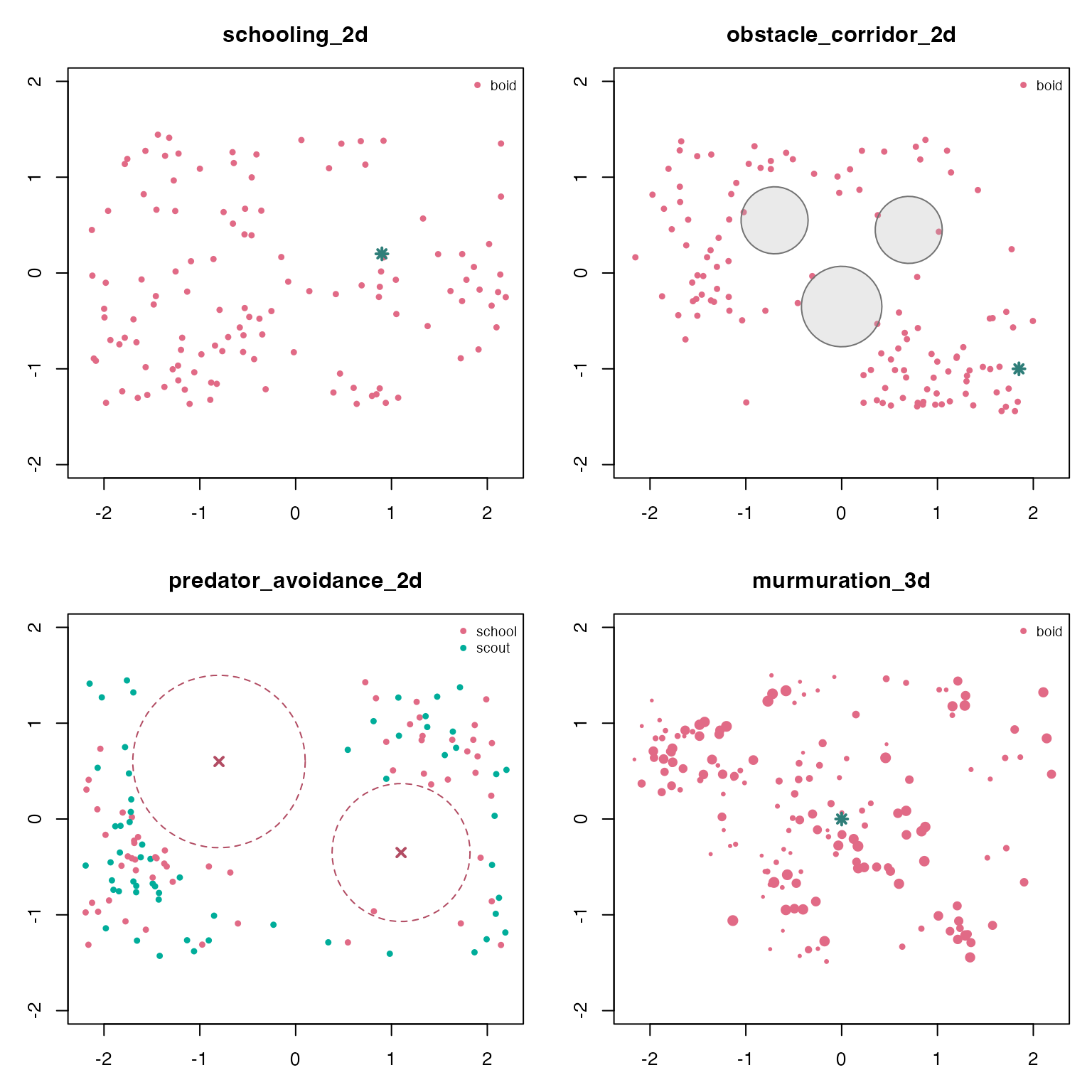
graphics::par(old_par)Hand off to ggWebGL
When ggWebGL 0.4.0 or later is installed, the same
simulation object can be converted into a timeline-aware WebGL
specification. The adapter keeps current boids visually dominant, draws
recent history as faint trails, colours velocity vectors by species by
default, and includes visible rings for obstacles and predator influence
zones. This step is optional and leaves the core simulation object
renderer-neutral.
if (requireNamespace("ggWebGL", quietly = TRUE) &&
    utils::packageVersion("ggWebGL") >= "0.4.0") {
  ggWebGL::ggWebGL(
    as_ggwebgl_spec(sims$mixed_species_3d, trail_length = 30),
    height = 520
  )
}