Recorded boids frames can be used as generative drawing material. This vignette keeps the simulation renderer-neutral, then turns frame tables into static artworks with base R graphics.
The vignette has two parts:
- Foundational swarm-art recipes, which introduce trails, time layering, negative space, and depth coding.
- Spectacular swarm-art examples, which combine richer initial states, obstacle fields, predator fields, and projected 3D simulations.
The examples use base R graphics so the vignette builds without
optional visualization packages. Optional WebGL export chunks are not
evaluated during package checks and write only to
tempdir().
Shared helpers
frame_table <- function(sim) {
  frames <- as.data.frame(sim)
  frames[order(frames$id, frames$frame), , drop = FALSE]
}

final_frame <- function(sim) {
  frames <- as.data.frame(sim)
  frames[frames$frame == max(frames$frame), , drop = FALSE]
}

world_limits <- function(sim) {
  list(
    xlim = sim$world$bounds["x", ],
    ylim = sim$world$bounds["y", ]
  )
}

draw_empty_canvas <- function(sim, title = "") {
  lim <- world_limits(sim)
  graphics::plot(
    NA_real_, NA_real_,
    xlim = lim$xlim,
    ylim = lim$ylim,
    asp = 1,
    axes = FALSE,
    xlab = "",
    ylab = "",
    main = title
  )
}

fade_palette <- function(n, palette = "Inferno") {
  grDevices::hcl.colors(n, palette)
}

scale01 <- function(x) {
  r <- range(x, finite = TRUE)
  if (!all(is.finite(r)) || diff(r) == 0) return(rep(0.5, length(x)))
  (x - r[1]) / diff(r)
}

speed_palette <- function(x, palette = "Inferno") {
  grDevices::hcl.colors(64, palette)[pmax(1L, pmin(64L, floor(1 + 63 * scale01(x))))]
}

select_trails <- function(sim, n_ids = 80L, every = 1L) {
  frames <- as.data.frame(sim)
  ids <- unique(frames$id)
  ids <- ids[seq_len(min(length(ids), n_ids))]
  frames <- frames[frames$id %in% ids & frames$frame %% every == 0L, , drop = FALSE]
  frames[order(frames$id, frames$frame), , drop = FALSE]
}

draw_trail_art <- function(sim,
                           title,
                           n_ids = 90L,
                           every = 1L,
                           palette = "Inferno",
                           trail_alpha = 0.16,
                           point_alpha = 0.82,
                           point_cex = 0.55) {
  trails <- select_trails(sim, n_ids = n_ids, every = every)
  final <- final_frame(sim)
  lim <- world_limits(sim)

  graphics::plot(
    NA_real_, NA_real_,
    xlim = lim$xlim,
    ylim = lim$ylim,
    asp = 1,
    axes = FALSE,
    xlab = "",
    ylab = "",
    main = title
  )

  cols <- speed_palette(trails$speed, palette = palette)
  ids <- split(seq_len(nrow(trails)), trails$id)
  for (ii in ids) {
    if (length(ii) > 1L) {
      graphics::lines(
        trails$x[ii], trails$y[ii],
        col = grDevices::adjustcolor(cols[ii[length(ii)]], alpha.f = trail_alpha),
        lwd = 0.8
      )
    }
  }

  graphics::points(
    final$x, final$y,
    pch = 16,
    cex = point_cex,
    col = grDevices::adjustcolor(speed_palette(final$speed, palette), alpha.f = point_alpha)
  )
}

radial_state <- function(n,
                         bounds,
                         species = "boid",
                         radius = 1.15,
                         twist = 3.0,
                         inward = 0.15) {
  i <- seq_len(n)
  theta <- 2 * pi * i / n
  r <- radius * sqrt(i / n)
  positions <- cbind(
    r * cos(theta),
    r * sin(theta)
  )
  velocities <- cbind(
    -sin(theta) + inward * cos(twist * theta),
    cos(theta) + inward * sin(twist * theta)
  )
  boids_state(
    n,
    "2d",
    bounds = bounds,
    positions = positions,
    velocities = velocities,
    species = species
  )
}
Foundational swarm-art recipes
This section introduces compact recipes for using recorded frames as drawing material. These examples favour simple simulation calls and short plotting code.
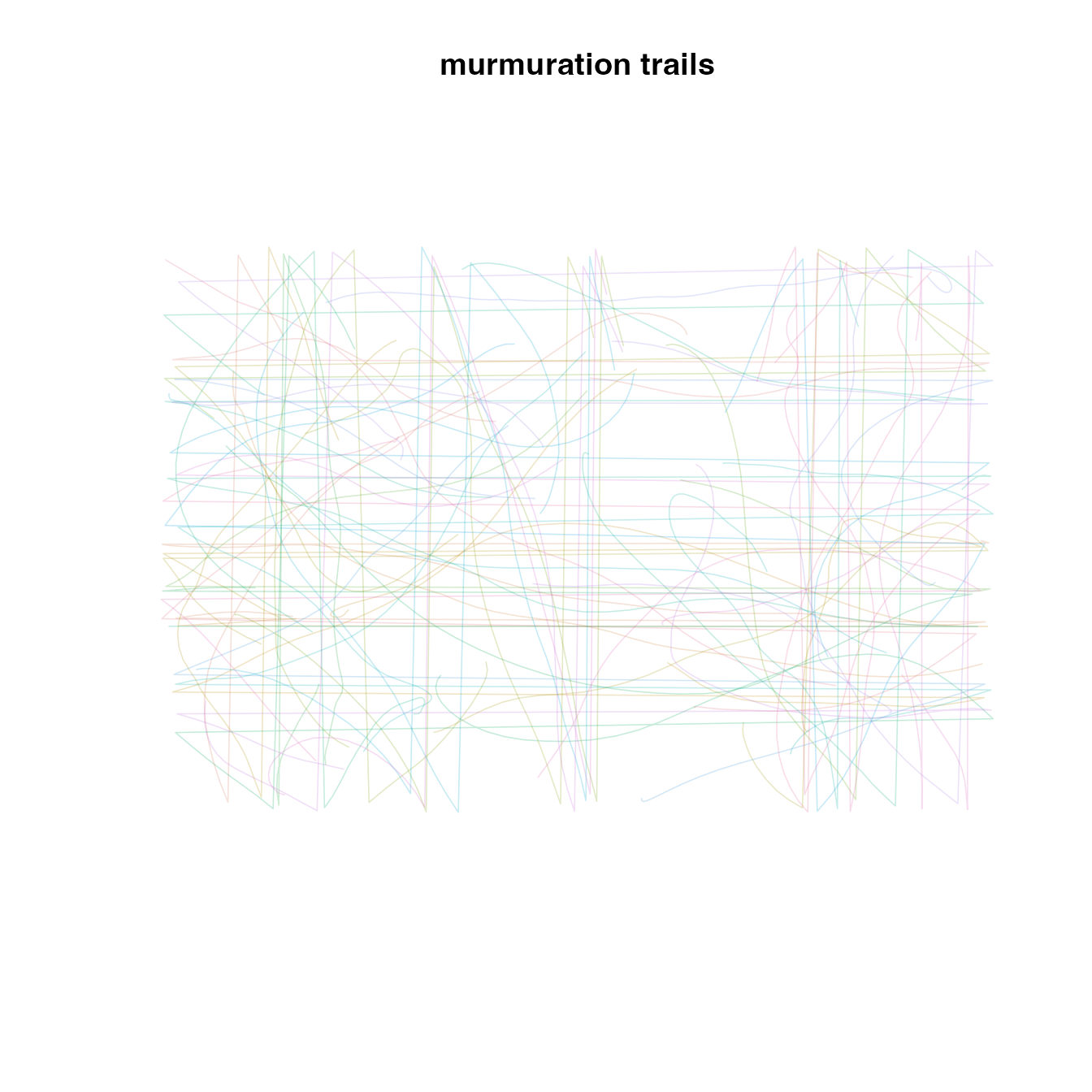
Trail drawing
Line trails turn motion into a dense drawing. The example below draws only a subset of boids so individual paths remain visible.
trail_sim <- boids_scenario(
  "murmuration_3d",
  n = 140,
  steps = 95,
  record_every = 2,
  seed = 710
)

trail_frames <- frame_table(trail_sim)
keep_ids <- unique(trail_frames$id)[seq(1, length(unique(trail_frames$id)), by = 3)]
trail_frames <- trail_frames[trail_frames$id %in% keep_ids, , drop = FALSE]
draw_empty_canvas(trail_sim, "murmuration trails")
ids <- unique(trail_frames$id)
cols <- grDevices::adjustcolor(fade_palette(length(ids), "Dark 3"), alpha.f = 0.22)
for (i in seq_along(ids)) {
  path <- trail_frames[trail_frames$id == ids[i], , drop = FALSE]
  graphics::lines(path$x, path$y, col = cols[i], lwd = 0.8)
}
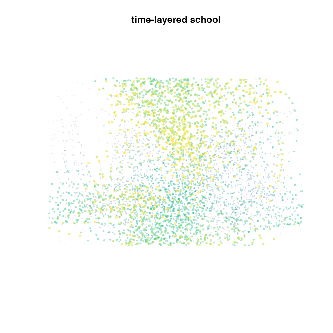
Time-layered particles
A different style keeps all boids but draws successive frames with increasing opacity and size. Recent frames become the bright foreground.
particle_sim <- boids_scenario(
  "schooling_2d",
  n = 180,
  steps = 75,
  record_every = 3,
  seed = 720
)
particle_frames <- as.data.frame(particle_sim)
frames <- sort(unique(particle_frames$frame))
draw_empty_canvas(particle_sim, "time-layered school")
frame_cols <- vapply(
  seq_along(frames),
  function(i) {
    grDevices::adjustcolor(
      fade_palette(length(frames), "Viridis")[i],
      alpha.f = seq(0.06, 0.55, length.out = length(frames))[i]
    )
  },
  character(1)
)
for (i in seq_along(frames)) {
  layer <- particle_frames[particle_frames$frame == frames[i], , drop = FALSE]
  graphics::points(layer$x, layer$y, pch = 16, cex = 0.25 + 0.45 * i / length(frames), col = frame_cols[i])
}
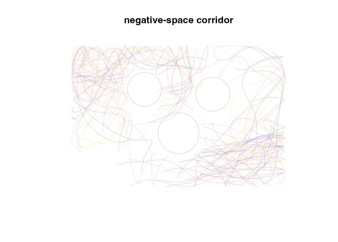
Negative-space obstacles
Obstacle and predator avoidance can produce visual gaps. Here the obstacles are drawn as quiet negative-space forms under the flock traces.
negative_sim <- boids_scenario(
  "obstacle_corridor_2d",
  n = 170,
  steps = 85,
  record_every = 3,
  seed = 730
)
negative_frames <- frame_table(negative_sim)
negative_ids <- unique(negative_frames$id)[seq(1, length(unique(negative_frames$id)), by = 2)]
negative_frames <- negative_frames[negative_frames$id %in% negative_ids, , drop = FALSE]
draw_empty_canvas(negative_sim, "negative-space corridor")
for (i in seq_len(nrow(negative_sim$world$obstacles))) {
  graphics::symbols(
    negative_sim$world$obstacles$x[i],
    negative_sim$world$obstacles$y[i],
    circles = negative_sim$world$obstacles$radius[i],
    inches = FALSE,
    add = TRUE,
    bg = "white",
    fg = "gray85"
  )
}
cols <- grDevices::adjustcolor(fade_palette(length(negative_ids), "Plasma"), alpha.f = 0.18)
for (i in seq_along(negative_ids)) {
  path <- negative_frames[negative_frames$id == negative_ids[i], , drop = FALSE]
  graphics::lines(path$x, path$y, col = cols[i], lwd = 0.9)
}
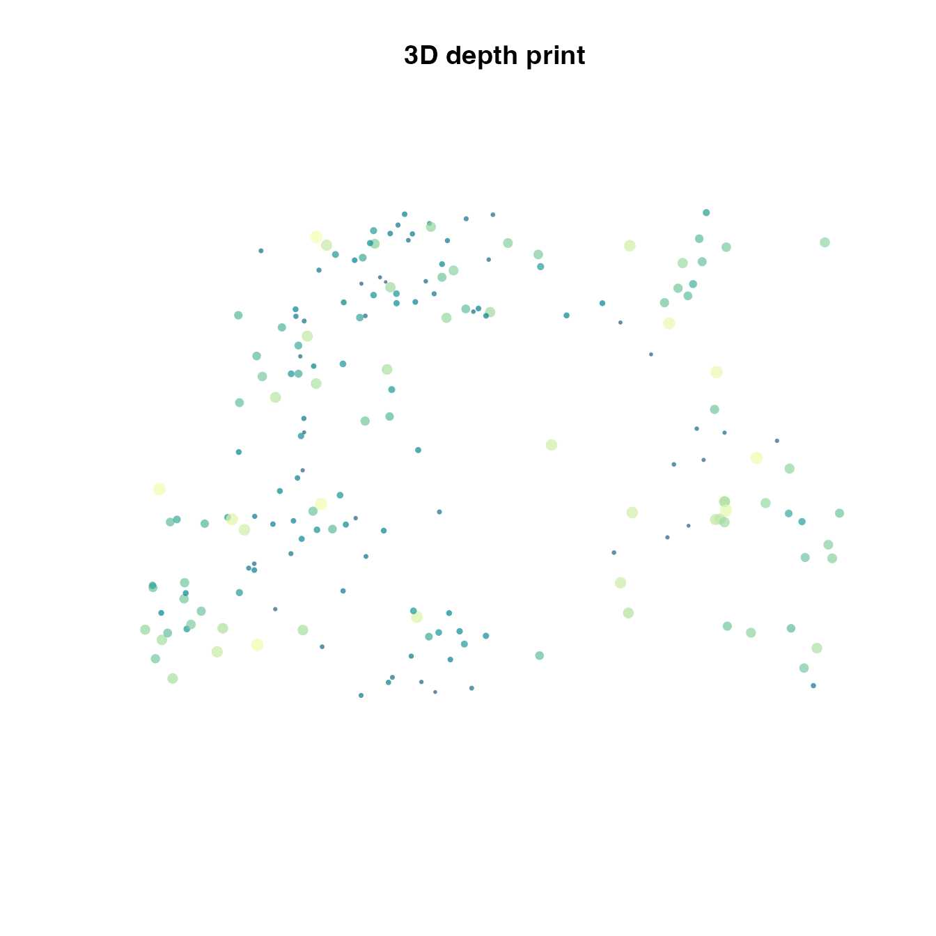
Depth as colour
For 3D simulations, z can drive colour or point size in a 2D projection. This creates a depth print without needing a 3D renderer.
depth_sim <- boids_scenario(
  "mixed_species_3d",
  n = 190,
  steps = 70,
  record_every = 5,
  seed = 740
)
depth_final <- final_frame(depth_sim)
depth_rank <- scale01(depth_final$z)
draw_empty_canvas(depth_sim, "3D depth print")
depth_cols <- fade_palette(100, "BluYl")
graphics::points(
  depth_final$x,
  depth_final$y,
  pch = 16,
  cex = 0.35 + 0.9 * depth_rank,
  col = grDevices::adjustcolor(depth_cols[pmax(1, ceiling(depth_rank * 99))], alpha.f = 0.7)
)
Spectacular swarm-art examples
This section uses larger swarms, custom initial conditions, speed-coded trails, and projected 3D motion to create more dramatic static artworks.
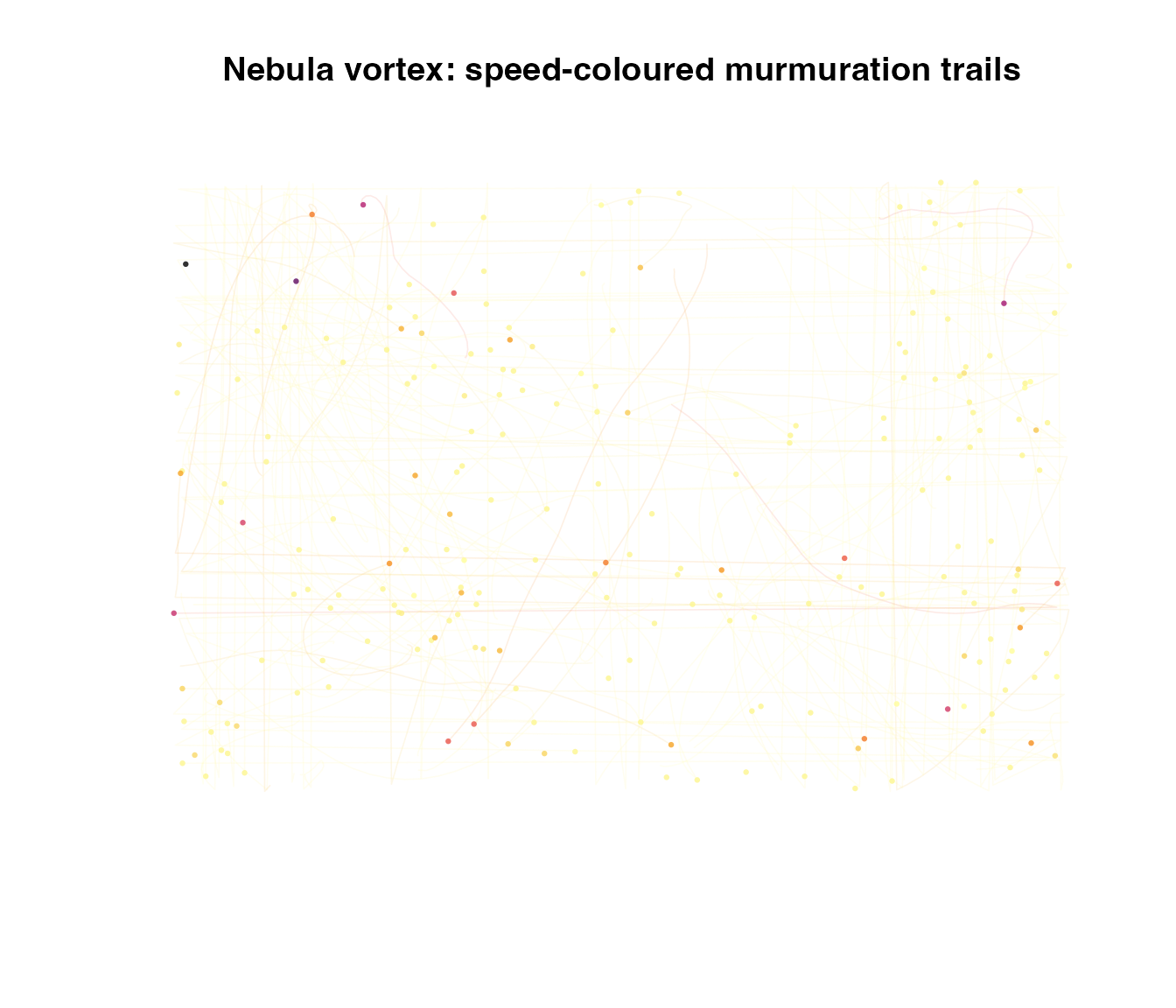
Nebula vortex
A dense 3D murmuration is projected from above. The colour encodes speed and the trails reveal the invisible flow field.
nebula <- boids_scenario(
  "murmuration_3d",
  n = 220,
  steps = 55,
  record_every = 2,
  seed = 2401
)

draw_trail_art(
  nebula,
  "Nebula vortex: speed-coloured murmuration trails",
  n_ids = 120,
  every = 2,
  palette = "Inferno",
  trail_alpha = 0.13,
  point_cex = 0.45
)
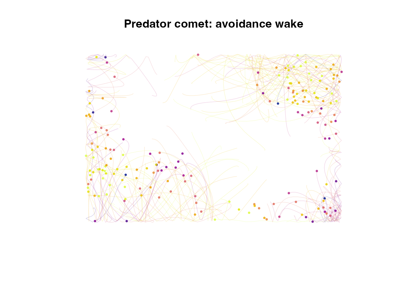
Predator comet
A predator field cuts through a 2D school. The swarm leaves a comet-like wake as boids avoid the danger zone while preserving local alignment.
comet <- boids_scenario(
  "predator_avoidance_2d",
  n = 180,
  steps = 65,
  record_every = 2,
  seed = 2402
)

draw_trail_art(
  comet,
  "Predator comet: avoidance wake",
  n_ids = 110,
  every = 2,
  palette = "Plasma",
  trail_alpha = 0.18,
  point_cex = 0.55
)
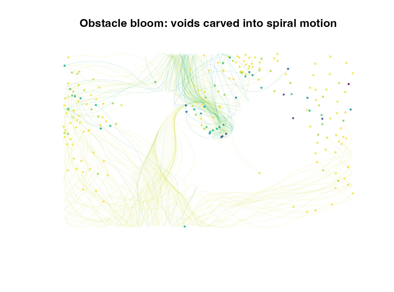
Obstacle bloom
The boids start on a deterministic spiral and are pulled toward a goal while three obstacle discs carve voids in the drawing.
bloom_bounds <- matrix(
  c(-2.4, -1.45, 2.4, 1.45),
  ncol = 2,
  dimnames = list(c("x", "y"), c("min", "max"))
)

bloom <- simulate_boids(
  radial_state(
    210,
    bloom_bounds,
    species = rep(c("amber", "blue", "white"), length.out = 210),
    radius = 1.22,
    twist = 5.0,
    inward = 0.28
  ),
  boids_world(
    "2d",
    bounds = bloom_bounds,
    boundary = "reflect",
    obstacles = data.frame(
      x = c(-0.72, 0.02, 0.82),
      y = c(0.48, -0.38, 0.36),
      radius = c(0.28, 0.40, 0.30)
    ),
    attractors = data.frame(x = 1.95, y = -0.78, strength = 0.72)
  ),
  boids_params(
    "2d",
    separation_weight = 1.36,
    alignment_weight = 0.98,
    cohesion_weight = 0.70,
    obstacle_weight = 2.80,
    goal_weight = 0.24,
    max_speed = 1.22,
    max_force = 0.11,
    noise = 0.001
  ),
  steps = 70,
  record_every = 2,
  seed = 2403
)

draw_trail_art(
  bloom,
  "Obstacle bloom: voids carved into spiral motion",
  n_ids = 140,
  every = 2,
  palette = "Viridis",
  trail_alpha = 0.16,
  point_cex = 0.50
)
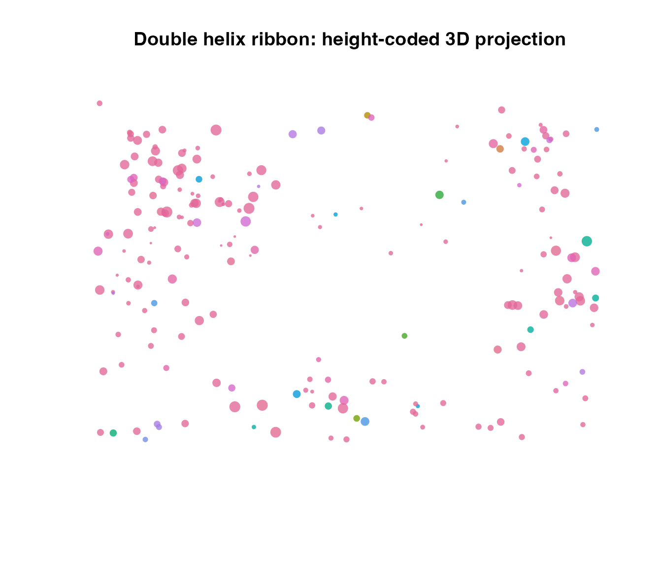
Double helix ribbon
A full 3D mixed-species swarm can be turned into a ribbon-like image by mapping height to point size. The plot is still a static base-R projection; no WebGL is required to build the vignette.
ribbon <- boids_scenario(
  "mixed_species_3d",
  n = 210,
  steps = 60,
  record_every = 2,
  seed = 2404
)

ribbon_final <- final_frame(ribbon)
z_size <- 0.35 + 1.20 * scale01(ribbon_final$z)

graphics::plot(
  ribbon_final$x, ribbon_final$y,
  xlim = ribbon$world$bounds["x", ],
  ylim = ribbon$world$bounds["y", ],
  asp = 1,
  axes = FALSE,
  xlab = "",
  ylab = "",
  main = "Double helix ribbon: height-coded 3D projection",
  pch = 16,
  cex = z_size,
  col = grDevices::adjustcolor(speed_palette(ribbon_final$speed, "Dark 3"), alpha.f = 0.78)
)
Exporting art
Use normal graphics devices to export a static artwork. Examples that write files must use temporary locations so package checks do not write into the package directory or the user’s working directory.
outfile <- file.path(tempdir(), "swarm-art.png")
png(outfile, width = 1800, height = 1800, res = 220)
draw_empty_canvas(trail_sim, "murmuration trails")
for (i in seq_along(ids)) {
  path <- trail_frames[trail_frames$id == ids[i], , drop = FALSE]
  graphics::lines(path$x, path$y, col = cols[i], lwd = 0.8)
}
dev.off()
utils::browseURL(outfile)
The same frame table can also be sent to ggWebGL when an
animated artwork is preferable. This optional block is not evaluated
during checks and also writes only to tempdir().
if (requireNamespace("ggWebGL", quietly = TRUE) &&
    utils::packageVersion("ggWebGL") >= "0.4.0" &&
    requireNamespace("htmlwidgets", quietly = TRUE)) {
  spec <- as_ggwebgl_spec(
    depth_sim,
    trail_length = 30,
    vector_mode = "sampled",
    vector_every = 18,
    shader = "density_splat"
  )
  spec$render$timeline$autoplay <- TRUE
  widget <- ggWebGL::ggWebGL(spec, height = 540)

  outfile <- file.path(tempdir(), "boids4R_depth_art.html")
  htmlwidgets::saveWidget(widget, outfile, selfcontained = FALSE)
  utils::browseURL(outfile)
}
Design notes
These examples are intentionally renderer-neutral. The simulation
objects are ordinary boids_simulation values and the art
helpers consume only the recorded frame data. This keeps the examples
portable for CRAN checks while still making it straightforward to hand
the same frames to WebGL renderers for interactive presentations.