Using the networkABC package

Abstract

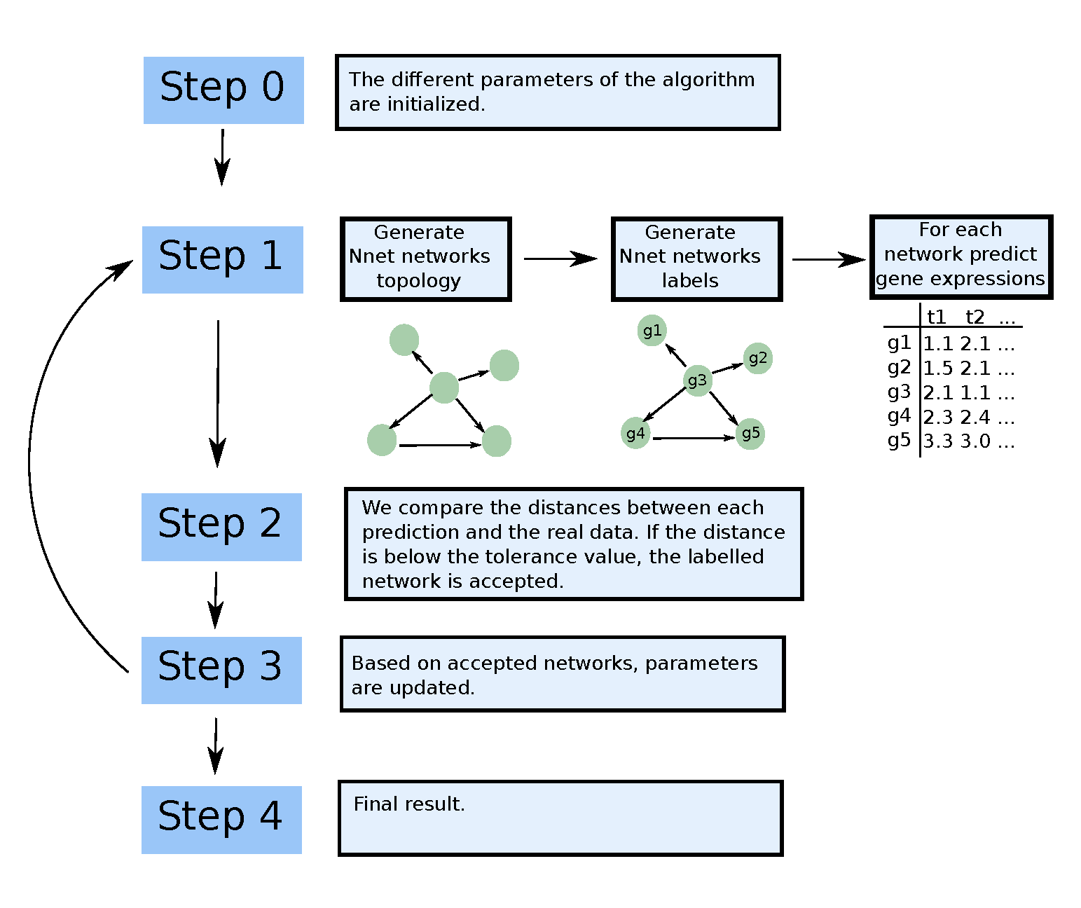
Elucidating gene regulatory network is an important step towards under- standing the normal cell physiology and complex pathological phenotype. Reverse- engineering consists in using gene expression over time or over different experimental conditions to discover the structure of the gene network in a targeted cellular process. The fact that gene expression data are usually noisy, highly correlated, and have high dimensionality explains the need for specific statistical methods to reverse engineer the underlying network. Among known methods, Approximate Bayesian Computation (ABC) algorithms have not been very well studied. Due to the computational overhead their application is also limited to a small number of genes. In this work we have developed a new multi-level ABC approach that has less computational cost. At the first level, the method captures the global properties of the network, such as scale-freeness and cluster- ing coefficients, whereas the second level is targeted to capture local properties, including the probability of each couple of genes being linked.

Overview

Steps of the network ABC package.

Generation of a network topology

Load the networkABC package.

library(networkABC)

Examples and checks

To generate a network, the number of node and the targeted clustering coefficient should be specified. For example, the following produces a network with 100 nodes and a targeted clustering coefficient of 0.33 :

net<-network_gen(100,0.33)

Then, we can plot the network :

require(network)
plot(network(net$network))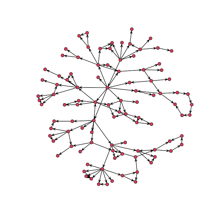

Here is a simulation to show that the algorithm produces networks with a clustering coefficient close to the targeted one

f<-function(a){
  a<-a[!is.nan(a)]
}

We generate 500 networks with 500 nodes with a targeted clustering coefficient of 0.33

set.seed(1234)
clco<-rep(0,500)
for(i in 1:500){
  N<-network_gen(500,.33)$net
  N<-N+t(N)
  clco[i]<-mean(f(abs(networkABC::clusteringCoefficient(N))))
}

Here is the result :

mean(clco)
#> [1] 0.3306789

sd(clco)
#> [1] 0.02874285

ggplot2::qplot(clco)

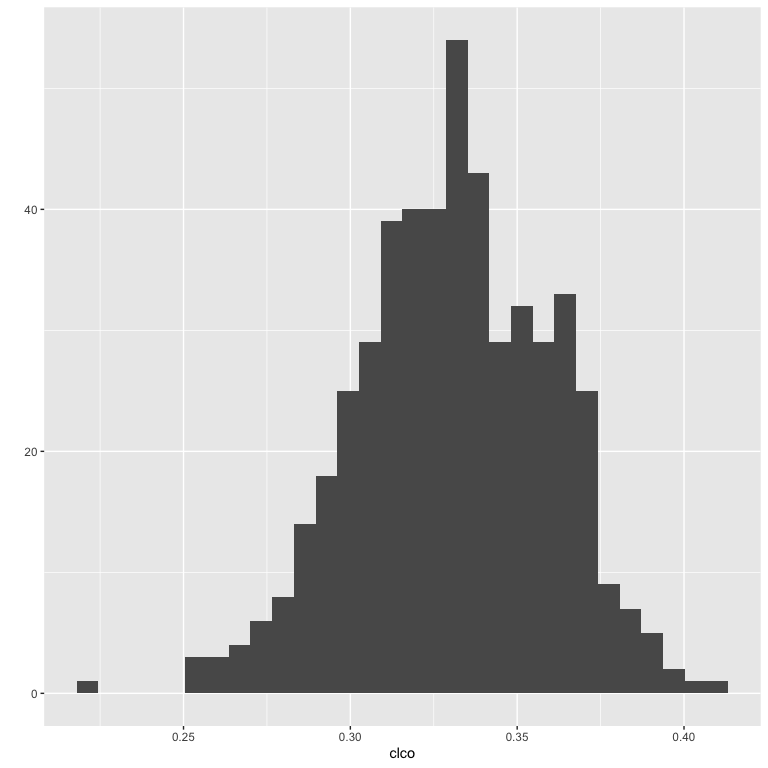
Notice that the algorithm cannot reach all desired values of clustering coefficients, because the network has to be scalefree.

For example, a clustering coefficient of 1 implies that every couple of nodes are linked together ; such a network is obviously not scale-free.

Details about the algorithm

This algorithm is partially based on the algorithm by Di Camillo, Barbara, Gianna Toffolo, and Claudio Cobelli. ”A gene network simulator to assess reverse engineering algorithms.” Annals of the New York Academy of Sciences.

Let us call \(V\) the set of nodes to be connected in the graph \(G\) at the current iteration \(t\) and \(H\) the set of nodes to be connected at iteration \(t + 1\). \(V\) is initialized as \(V = {1, ...,N}\), that is, with all the \(N\) nodes in \(G\), whereas \(H\) is initialized as the empty set \(H\). Nodes are then linked to each other through an iterative procedure, which consists of three main steps, explained in detail below. 1. Three candidate modules are generated. The structure is sampled from a pool of motifs, with possibility of random changes. The number of node of the module is set at random. In this algorithm we have : feedback motif, feedforward motifs and loops. 2. A score is assigned to each module, and one of the three modules is sampled with probability proportional to this score; let us denote the sampled module by M and the number of its nodes by \(m\). 3. \(m\) nodes are sampled from \(V\) and linked to each other in the graph \(G\), according to the selected module structure \(M\); \(V\) is updated by deleting the m sampled nodes; \(H\) is updated by adding the nodes. At the end of this process, \(V\) is empty whereas \(H\) is composed of a lot of motifs. To link the motifs together, we have to choose one node in each motif that is the first position. This set of nodes is then considered as set \(V\) .

Running the ABC algorithm

The simpliest way

set.seed(123)
M<-matrix(rnorm(30),10,3)
result<-abc(data=M)
#> First run of abc to find tolerance
#> ===============================
#> Iteration=1
#> Accepted:1000
#> Probabilities of clustering coefficients:
#> 0.325000 0.349000 0.326000 
#> Tolerance value
#>       5% 
#> 4.523488 
#> ===============================
#> Beginning main run of abc
#> ===============================
#> Iteration=1
#> Accepted:45
#> Probabilities of clustering coefficients:
#> 0.488889 0.311111 0.200000 
#> ===============================
#> Iteration=2
#> Accepted:109
#> Probabilities of clustering coefficients:
#> 0.522936 0.266055 0.211009 
#> ===============================
#> Iteration=3
#> Accepted:139
#> Probabilities of clustering coefficients:
#> 0.654676 0.201439 0.143885 
#> ===============================
#> Iteration=4
#> Accepted:163
#> Probabilities of clustering coefficients:
#> 0.705521 0.196319 0.098160 
#> ===============================
#> Iteration=5
#> Accepted:154
#> Probabilities of clustering coefficients:
#> 0.753247 0.181818 0.064935 
#> ===============================
#> Iteration=6
#> Accepted:210
#> Probabilities of clustering coefficients:
#> 0.819048 0.142857 0.038095 
#> ===============================
#> Iteration=7
#> Accepted:200
#> Probabilities of clustering coefficients:
#> 0.860000 0.120000 0.020000 
#> ===============================
#> Iteration=8
#> Accepted:163
#> Probabilities of clustering coefficients:
#> 0.865031 0.110429 0.024540 
#> ===============================
#> Iteration=9
#> Accepted:232
#> Probabilities of clustering coefficients:
#> 0.909483 0.077586 0.012931 
#> ===============================
#> Iteration=10
#> Accepted:238
#> Probabilities of clustering coefficients:
#> 0.907563 0.079832 0.012605

We can plot the results in three different ways :

networkABC::showHp(result)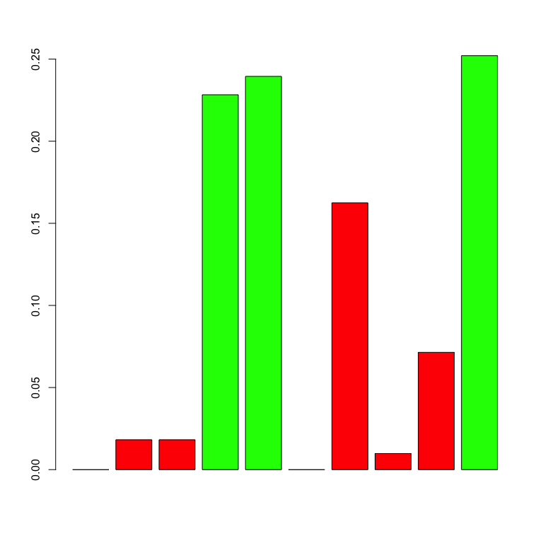

#>   gene.hubs hubs.proba
#> 1         4  0.2282913
#> 2         5  0.2394958
#> 3        10  0.2521008

This plot show the probabilities for each gene of being a hub. The following shows the probability for each couple of genes of being linked :

showNp(result)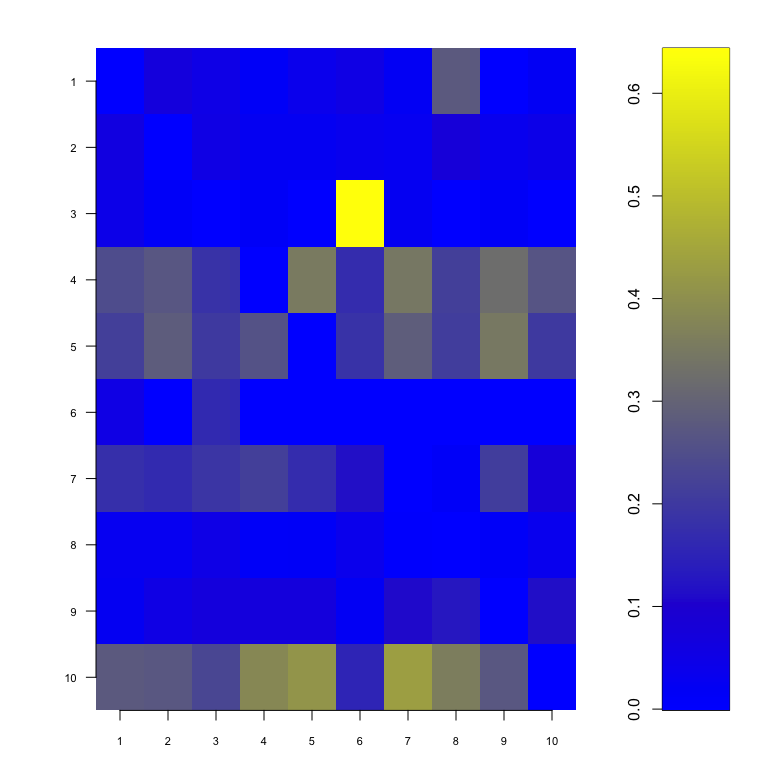

Specifying a probability cutoff (the minimal probability for which we can say that two genes are linked), we can plot the network :

showNetwork(result,0.3)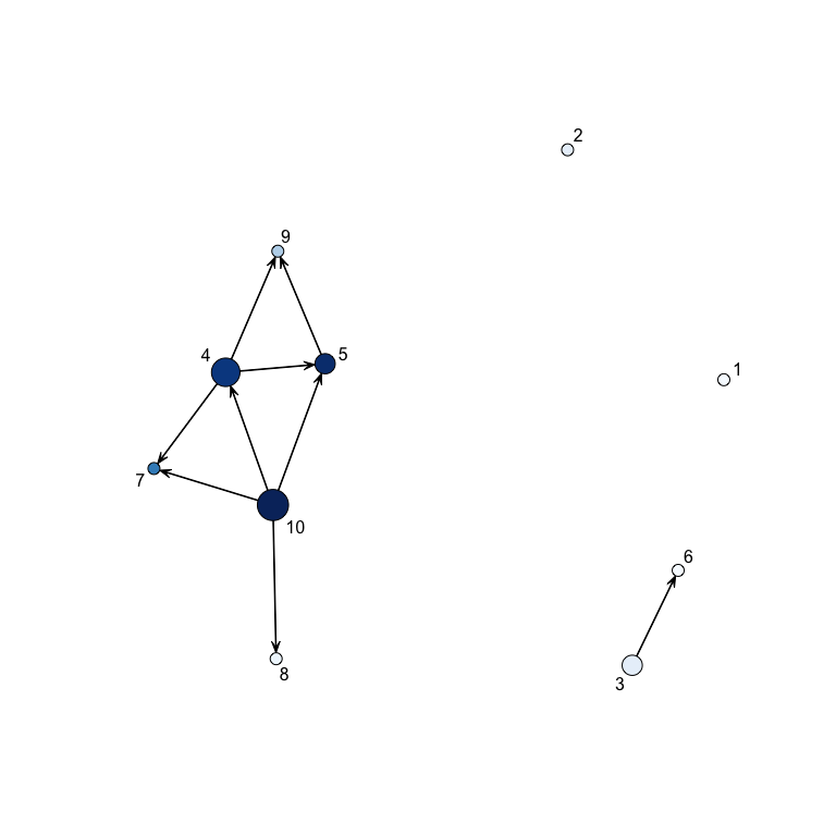

In this plot, the diameter of a node increases with the number of its children whereas the color is a function of the probability for each gene of being a hub.

You can also have a look on the error :

hist(result$dist)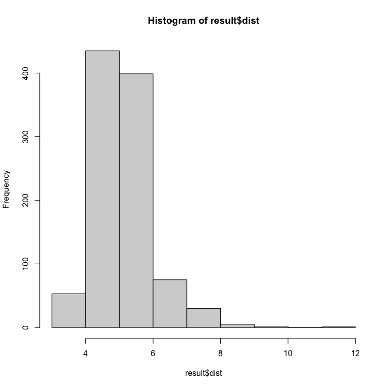

Using ABC algorithm with full options

You can specify all the arguments of the ABC function: more details in the help manual.

For example :

result<-abc(data=M,
            clust_coeffs=0.33, #you can specify more than one clustering coefficient
            tolerance=3.5, #maximal distance between simulated and real data
            # to accept the network
            number_hubs=3,#the number of hubs
            iterations=10, #number of iterations
            number_networks=1000000,#number of network simulated at each iteration
            hub_probs=NA,#specify the a priori probabilty for each gene to be a hub
            neighbour_probs=NA,#specify the a priori probability for each couple
            #of gene to be linked
            is_probs=1)#set this last option to one.

Frédéric Bertrand, Nicolas Jung, Myriam Maumy-Bertrand

2022-10-19