Partial Least Squares Regression for Beta Regression Models
The plsRbeta package
Frédéric Bertrand and Myriam Maumy-Bertrand
IRMA, labex IRMIA, Université de Strasbourg and CNRS. LIST3N, Université de technologie de Troyes.frederic.bertrand@lecnam.net
2025-09-20
Source:vignettes/tn_Insights.Rmd
tn_Insights.RmdAbstract
Many variables of interest, such as experimental results, yields or
economic indicators, are naturally expressed as rates, proportions or
indices whose values are necessarily between zero and one or more
generally two fixed values known in advance. Beta regression allows us
to model these data with a great deal of flexibility, since the density
functions of the Beta laws can take on a wide variety of forms. However,
like all usual regression models, it cannot be applied directly when the
predictors present multicollinearity problems or worse when they are
more numerous than the observations. These situations are frequently
encountered in chemistry, medicine, economics or marketing. To
circumvent this difficulty, we formulate an extension of PLS regression
for Beta regression models. This, along with several tools such as
cross-validation and bootstrap techniques, is available for the
R language in the plsRbeta library.
Introduction
PLS regression, the result of the NIPALS algorithm initially developed by Wold (Wold, 1966)1 and explained in detail by Tenenhaus (Tenenhaus, 1998)2, has already been successfully extended to generalized linear models by Bastien et al. (Bastien, 2005)3 and to Cox models by Bastien (Bastien 2008)4 and (Bastien 2015)5.
We proposed an extension of PLS regression to Beta regression models in Bertrand (2013)6. Indeed, the practical interest of the Beta distribution had been asserted several times, for example by Johnson et al. (Johnson, 1995)7 :
“Beta distributions are very versatile and a variety of uncertanties can be usefully modelled by them. This flexibility encourages its empirical use in a wide range of applications.”
Several articles have focused on the study of Beta regression and its properties. Let us mention in particular, the article by Ferrari and Cribari-Neto (Ferrari, 2004)8 for an introduction to these models and those by Kosmidis and Firth (Kosmidis, 2010)9, Simas et al. (Simas, 2010)10 and Grün et al. (Grün, 2012)11 for extensions or improvements of the estimation techniques of these models.
We will assume in the rest of the paper that the answer studied has values in the interval . The model we propose can of course be used as soon as the answer has values in a bounded interval , with fixed and known, by studying instead of .
PLS Beta Regression
Beta Regression
When it is non-zero, the density function of the law is given by : with , and the Euler gamma function. If follows a distribution, its expectation and variance are equal to : In order to be able to apply techniques similar to those used for generalized linear models by McCullagh and Nelder, Ferrari and Cribari-Neto (Ferrari, 2004)12 propose to rephrase the Beta law as follows. By posing and , i.e. and , the Equation () becomes : where . Thus is the mean value of the response and can be interpreted as a precision parameter since, for a fixed , the higher the value of , the smaller the variance of the response. With these new parameters, the density function given in Equation () is equal to :
It is not possible to apply directly the theory of the generalized linear model, as introduced by the founding article of Nelder and Wedderburn (Nelder, 1972)13 and then taken up again in the eponymous book of McCullagh and Nelder (McCullagh, 1995)14, because it is based on the use of a family of laws put in natural exponential form (NEF). However, as indicated by Morris (Morris, 1982)15, the family of beta laws, with the parameterization taken up by Ferrari and Cribari-Neto (Ferrari, 2004)16 and introduced above, is certainly a univariate exponential family but not a natural exponential family. Indeed, the latter are characterized by their variance function. But the variance function of this parameterization of the family of beta laws is already that of the natural exponential family formed by the binomial laws, hence the result. For the same reason, it is not possible to characterize, within the exponential families, the family of Beta distributions by means of their variance function.
Let , , be independent random variables distributed according to the density function given in Equation () of mean and unknown precision .
We obtain the Beta regression model by assuming that the mean of , , can be written : where is a vector of unknown regression parameters (), denoting the matrix transpose, and are the observations of the predictors with that are assumed to be known and fixed. Finally, is a strictly monotone, twice derivable, surjective link function defined on the interval and with values in . The variance of is a function of and thus depends on the value of the covariates. Therefore, the model automatically takes into account the possible lack of homoscedasticity.
There are several common choices for the link function . For example, the logit link , the probit link , with the distribution function of the centered and reduced normal distribution, the complementary log-log link , the log-log link . A detailed study of these links has been made by McCullagh and Nelder (McCullagh, 1995)17 and Atkinson (Atkinson, 1985)18 has proposed others. As usual, the use of the logit link makes it possible to interpret the exponential of the coefficients of the covariates in terms of the odds ratio.
PLS Regression
Consider the centered variables , , , , , . Let be the matrix of predictors , , , , . PLS regression is well known and exhaustively described by Höskuldsson (Höskuldsson, 1988)19, Wold et al. (Wold, 2001)20 and Tenenhaus (Tenenhaus, 1998)21. The classical presentation of PLS regression is in algorithmic form. We will only recall the elements that are useful for the following. PLS regression is a non-linear model which allows to construct orthogonal components obtained by maximizing the quantities . Let be the matrix formed by these components, we have : where is the vector of residuals and is the vector of component coefficients. By positing , where is the matrix of the coefficients of the variables in each component, we have the direct expression for the response using the predictors: Expanding the right-hand side of Equation~(), we obtain for each component of : being the number of components retained in the final model with , being in general much lower than the rank of and being equal to the number of variables contained in the matrix . The coefficients , where , following the notation with of Wold et al. (Wold, 2001)22, translate the relation between the vector and the variables through the components .
PLS Beta Regression
PLS Beta Regression of the response on the variables , , , , with components is written : where is the expectation of . The link is to be chosen among the links logit, probit, complementary log-log, log-log, Cauchit and log according to the type of data and the quality of the model fit to the data.
The algorithm for determining the PLS components of a Beta PLS regression model is as follows:
- Compute the first PLS component :
- Compute the coefficient of in the Beta regression of on for each predictor , .
- Norm the column vector : .
- Compute the component .
- Compute the second PLS component :
- Compute the coefficient of in the Beta regression of on and for each predictor , .
- Norm the column vector : .
- Compute the residual matrix of the linear regression of on .
- Compute the component .
- Express the component in terms of predictors : .
- We assume having constructed components , . We then compute the th PLS component :
- Compute the coefficient of in the Beta regression model of on , , $t_ldots, , and for each predictor , .
- Normalize the column vector : .
- Compute the residual matrix of the linear regression of on , , .
- Compute the component .
- Express the component in terms of predictors : .
Proposition
The PLS components are orthogonal.
It is easy to modify the previous algorithm to be able to handle incomplete datasets (Tenenhaus, 1998)23.
Bootstrap techniques, cross-validation and software implementation
Bootstrap techniques
We assume that we have retained the appropriate number of components of a Beta PLS regression model on , , , , . We propose the following algorithm to construct confidence intervals and significance tests for the predictors , , using bootstrap techniques. Let be the empirical distribution function given the matrix formed by the PLS components and the response .
- Step 1. Draw samples from .
- Step 2. For all , calculate : where is the th bootstrap sample, is the vector of component coefficients and is the vector of coefficients of the original predictors for this sample and finally is the fixed matrix of the weights of the predictors in the original model with components.
- Step 3. For each , let be the Monte Carlo approximation of the distribution function of the bootstrap statistic of . For each , whisker boxes and confidence intervals can be constructed using the percentiles of . A confidence interval can be defined as where and are the values obtained from the distribution function of the bootstrap statistic such that a nominal level of confidence of level is reached. In order to improve the quality of the confidence interval in terms of coverage rates, i.e., the ability of to provide the expected coverage rates, it is possible to use several construction techniques: normal, percentile, or (Efron 1993)24 or (Davison 1997)25. The resulting intervals are not intended to be used for multiple or pairwise comparisons and should be interpreted separately.
Strengths of the software implementation
The plsRbeta function library for the R
language implements PLS Beta regression models. It uses the Beta
regression implemented in the betareg (Cribari-Neto,
2010)26
function library for the R language to perform the
step.
- Beta PLS regression models with complete or incomplete data.
- Choice of the number of components thanks to different criteria AIC, BIC, modified , stop of significance of the component when none of the coefficients is significant in the model at a given level or by using a criterion estimated by cross validation.
- Repeated -fold cross-validation with complete or incomplete data. Tables 3 and 5 are examples of using cross-validation to determine the appropriate number of components.
- Bootstrapping predictor coefficients for Beta PLS regression models
with complete or incomplete data. Various interval constructions,
detailed in Efron and Tibshirani (Efron, 1993)27 or Davison and
Hinkley (Davison, 1997)28, are available and are based on the
boot(Canty, 2021)29 function library for theRlanguage. Figure 5 is an example of whisker boxes constructed from the bootstrap distribution of the coefficients of the predictors of a PLS Beta regression model. Figures 2, 3, and 6 are examples of using bootstrap techniques to establish the significance of the predictors of a PLS Beta regression model.
Selecting the number of components
A crucial problem for the correct use of PLS regression is the determination of the number of components. If, in the case of the original PLS regression, the criterion is extremely efficient, its good properties unfortunately disappear for the PLS generalized linear regression models. A simulation study is therefore necessary to determine a functional criterion to choose the number of components. We propose to compare the following criteria and (Cribari-Neto, 2010)30, Pearson’s , Pearson’s and pseudo- (Ferrari, 2004)31 or cumulative and criteria estimated by 5-group cross-validation (5-CV) or 10-group cross-validation (10-CV) (Bastien, 2005)32.
The following parameters were used for the simulation design.
- Number of individuals: 25, 50 and 100.
- Number of variables: 10, 25, 50 and 100.
- Number of components: 2, 4 and 6.
- dispersion : 2,5, 5, 10 and 15.
The algorithm used to create the simulated data is a direct adaptation of the algorithm of Li et al. (Li, 2002)33 which is itself a multivariate generalization of that of Naes and Martens (Naes, 1985)34. This type of generalization has already been used successfully in the case of PLS logistic regression models (Meyer, 2010)35.
Table 1 is an example of a result for 25 individuals, 10 variables, 2 components and a dispersion parameter equal to 2.5. For 100 simulated data sets, a maximum number of 6 components had to be calculated. The average number of components that could actually be computed, as well as the number of complete failures of the beta regression model fit are shown in Table 2. The abbreviations , , and indicate that the Beta regressions used to fit the Beta PLS regression are based on maximum likelihood, bias reduction, or bias correction (Kosmidis, 2010)36. The prefixes and mean that the value was obtained after cross-validation in or groups.
| Criterion | Mean | SD | Median | MAD | Criterion | Mean | SD | Median | MAD |
|---|---|---|---|---|---|---|---|---|---|
| 3.53 | 0.94 | 3.5 | 0.74 | 2.86 | 2.05 | 2 | 1.48 | ||
| 3.1 | 0.8 | 3 | 0 | 4.71 | 1.97 | 6 | 0 | ||
| 2.84 | 2.05 | 2 | 1.48 | 0 | 0 | 0 | 0 | ||
| 5.15 | 1.31 | 6 | 0 | 1.37 | 0.49 | 1 | 0 | ||
| 3.96 | 1.59 | 4 | 2.97 | 2.84 | 2.05 | 2 | 1.48 | ||
| 5.15 | 1.31 | 6 | 0 | 4.64 | 1.98 | 6 | 0 | ||
| 3.42 | 0.87 | 3 | 1.48 | 0.06 | 0.24 | 0 | 0 | ||
| 3.02 | 0.79 | 3 | 0 | 1.48 | 0.5 | 1 | 0 | ||
| 5.3 | 1.57 | 6 | 0 | 2.89 | 2.04 | 2 | 1.48 | ||
| 5.14 | 1.33 | 6 | 0 | 4.84 | 1.87 | 6 | 0 | ||
| 3.98 | 1.58 | 4 | 2.97 | 0.07 | 0.26 | 0 | 0 | ||
| 5.14 | 1.33 | 6 | 0 | 1.54 | 0.5 | 2 | 0 | ||
| 3.43 | 0.81 | 3 | 1.48 | 2.87 | 2.04 | 2 | 1.48 | ||
| 3.04 | 0.74 | 3 | 0 | 4.42 | 2.02 | 6 | 0 | ||
| 5.16 | 1.64 | 6 | 0 | 0.07 | 0.26 | 0 | 0 | ||
| 5.03 | 1.28 | 6 | 0 | 1.47 | 0.5 | 1 | 0 | ||
| 3.95 | 1.53 | 4 | 1.48 | 2.89 | 2.06 | 2 | 1.48 | ||
| 5.03 | 1.28 | 6 | 0 | 4.53 | 1.94 | 6 | 0 | ||
| 4.69 | 1.89 | 6 | 0 | 0.08 | 0.27 | 0 | 0 | ||
| 0 | 0 | 0 | 0 | 1.52 | 0.5 | 2 | 0 | ||
| 1.43 | 0.5 | 1 | 0 | 2.87 | 2.04 | 2 | 1.48 |
Note that the MAD is the median of the absolute deviations from the median. It is a robust indicator of dispersion naturally associated with the median. A value of 0 for the MAD means that in more than half of the simulations, the value chosen for the number of components is equal to the median value of all simulations.
In general, the results of the simulation study show that the (5-CV and 10-CV), already known for its surprising behavior in PLS logistic regression (Bastien, 2005)37, (Meyer, 2010)38, does not behave much better for the Beta PLS regression models. Maximizing the or pseudo- criteria, also proves inefficient. The and criteria systematically retain a few too many components. This tendency is also known in the case of the traditional PLS Regression (Kramer, 2011)39 as well as in the case of the Logistic PLS Regression (Meyer, 2010)40.
| Mean | SD | Median | MAD | Failures | |
|---|---|---|---|---|---|
| ML | 5.55 | 1.22 | 6 | 0 | 0 |
| BC | 5.52 | 1.24 | 6 | 0 | 0 |
| BR | 5.43 | 1.22 | 6 | 0 | 1 |
| ML (5-CV) | 5.59 | 1.17 | 6 | 0 | 1 |
| ML (10-CV) | 5.55 | 1.22 | 6 | 0 | 0 |
| BC (5-CV) | 5.63 | 1.08 | 6 | 0 | 2 |
| BC (10-CV) | 5.6 | 1.13 | 6 | 0 | 1 |
| BR (5-CV) | 5.62 | 1.09 | 6 | 0 | 4 |
| BR (10-CV) | 5.6 | 1.13 | 6 | 0 | 1 |
We find that the proposed PLS Beta Regression algorithm succeeds in extracting the maximum number of components requested very consistently and that the fit is impossible in only one of the 100 simulations for the BR technique. The cross-validation, on the other hand, is completed in 98.5 % of the simulations.
Example of application in medicine
Cancerous tumors represent one of the three main causes of death in the Western world. The understanding of the mechanisms of cancer pathologies is currently based on the study of the interrelationships of acquired genetic abnormalities, which appear in tissues during the process of cancerization. These abnormalities are frequently analyzed by allelotyping, allowing to determine for a more or less important number of gene sites, the presence or not of a modification of the number of copies of each gene. The multivariate description of these anomalies is informative about the carcinogenesis process. Furthermore, the set of these gene sites with or without abnormalities can be used to try to predict certain clinical or biological characteristics of the tumor such as the tumor cell count on biopsy of a lesion. Modeling in a statistical model of rate, variable whose space of variation is contained in the closed interval as predicted variable suggests the use of Beta regression. Furthermore, allelotyping data are characterized by frequent collinearity and a large proportion of missing data. Moreover, the data matrix often has dimensions such that , which makes the matrix non-invertible, posing difficulties in fitting a regression model. The PLS Beta regression that we have developed is therefore particularly well suited to deal with allelotyping data in the particular context of predicting a rate variable.
The example is that of allelotyping data obtained on a series of 93 patients with different types of lung cancer and with missing values. The predicted variable is the tumor cellularity rate of the intraoperative tumor specimen. The explanatory variables are composed of 56 binary variables indicating the presence of an abnormality on each of the 56 microsatellites and three clinical variables.
The selection of variables is very important in this example because it allows to define a subset of predictors, i.e. gene sites, able to predict the tumor cell rate. Indeed, cancer pathologies are acquired genetic pathologies and some of these anomalies are the cause and others the consequence of the tumor pathology. Moreover, the information contained in the different microsatellite gene sites is potentially redundant. Variable selection, separating variables that probably play a driving role in tumor development from variables that merely reflect random background noise induced by abnormalities caused by tumor development, is therefore an indispensable aid to understanding the underlying mechanisms of tumorigenesis.
Table 3 summarizes the values of different criteria used to determine the number of components to be used to properly model the allelotype data with BR and a logit link.
| Nb of Comp. | 0 | 1 | 2 | 3 | 4 | 5 | 6 | 7 | 8 | 9 |
|---|---|---|---|---|---|---|---|---|---|---|
| AIC | ||||||||||
| BIC | ||||||||||
| Pred Sig | ||||||||||
| (5-CV) | ||||||||||
| Pearson | ||||||||||
| pseudo- | ||||||||||
| Pearson |
The stopping criterion as soon as there is no significant predictor would lead us to choose 6 components. This choice is confirmed by the pseudo- or criteria for which a kink appears from 6 components.
The BIC criterion invites us to choose 8 components and the AIC criterion an even higher number. During the simulation study, we noticed that these criteria are liberal and generally retain a few too many components.
Depending on the criteria, 6 or 8 components should be retained for a logit link. Taking into account the previous simulation study, we decide to retain 6 components. The same study was performed with the BC method or a log-log link and leads to the same conclusions.
Confidence intervals are then obtained for each of the predictors using bootstrap samples of size 1000 and the normal, basic, percentile or techniques.
The use of bootstrap techniques to establish the significance of the predictors of a PLS Beta regression model is illustrated in Figure 2 for the case of the 6-component model with the BR bias reduction technique.
In the end, we use the technique, known for its good properties, to select the variables that are significant at the 5 % threshold by retaining those for which the confidence interval does not contain 0, as shown in Figure 3 for the case of the 6-component model with the BR bias reduction technique.
Thus, we retain the variables in Table 4 as having a significant effect on the tumor cellularity rate of the intraoperative tumor specimen. We find that the two techniques for dealing with the Beta regression bias have results that differ only in the single variable EGF3, significant at the threshold for the BC technique and not for the BR technique.
| Nb Comp | Significant Variables | |||||
|---|---|---|---|---|---|---|
| 6 components | P4 | C3M | RB | FL7A | W2 | W4 |
| MT4 | HLA | HLD | HLB | EA3 | EA2 | |
| Bias Correction | EGF2 | EGF3 | FL7B | VSFGFR3 | VSTOP1 | VSTOP2A |
| VSEGFR | AFRAEGFR | SRXRA | SMT | SHL | SEB | |
| 6 components | P4 | C3M | RB | FL7A | W2 | W4 |
| MT4 | HLA | HLD | HLB | EA3 | EA2 | |
| Bias Reduction | EGF2 | FL7B | VSFGFR3 | VSTOP1 | VSTOP2A | VSEGFR |
| AFRAEGFR | SRXRA | SMT | SHL | SEB |
Figure 4 allows us to evaluate the stability of the significant variables selected by the bootstrap technique for a number of components varying from 1 to 6 and the two techniques BC and BR for fitting the Beta regression model.
data(TxTum)

TxTum.mod.bootBR6 <- bootplsbeta(plsRbeta(formula=I(CELTUMCO/100)~.,data=TxTum,nt=6,modele="pls-beta",type="BR"), sim="ordinary", stype="i", R=1000)
#save(TxTum.mod.bootBR6,file="TxTum.mod.bootBR6.Rdata")
data("TxTum.mod.bootBR6")
temp.ci <- suppressWarnings(plsRglm::confints.bootpls(TxTum.mod.bootBR6))
boxplots.bootpls(TxTum.mod.bootBR6,indices = 2:nrow(temp.ci))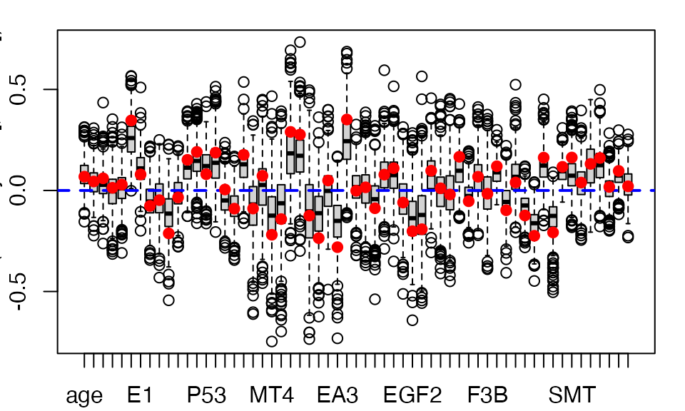
Figure 1. Boxplot of bootstrap distributions, 6 components BR.
plsRglm::plots.confints.bootpls(temp.ci,prednames=TRUE,indices = 2:nrow(temp.ci))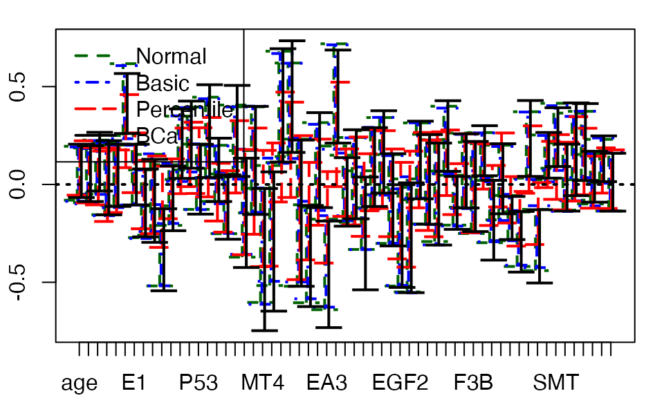
Figure 2. Bootstrap 95% confidence intervals, 6 components BR.
ind_BCa_nt6BR <- (temp.ci[,7]<0&temp.ci[,8]<0)|(temp.ci[,7]>0&temp.ci[,8]>0)
rownames(temp.ci)[ind_BCa_nt6BR]
#>  [1] "P4"       "C3M"      "RB"       "FL7A"     "W2"       "W4"
#>  [7] "MT4"      "HLA"      "HLD"      "HLB"      "EA3"      "EA2"
#> [13] "EGF2"     "FL7B"     "VSFGFR3"  "VSTOP1"   "VSTOP2A"  "VSEGFR"
#> [19] "AFRAEGFR" "SRXRA"    "SMT"      "SHL"      "SEB"
plsRglm::plots.confints.bootpls(temp.ci,prednames=TRUE,indices = (2:nrow(temp.ci))[ind_BCa_nt6BR[-1]],articlestyle=FALSE,legendpos="topright")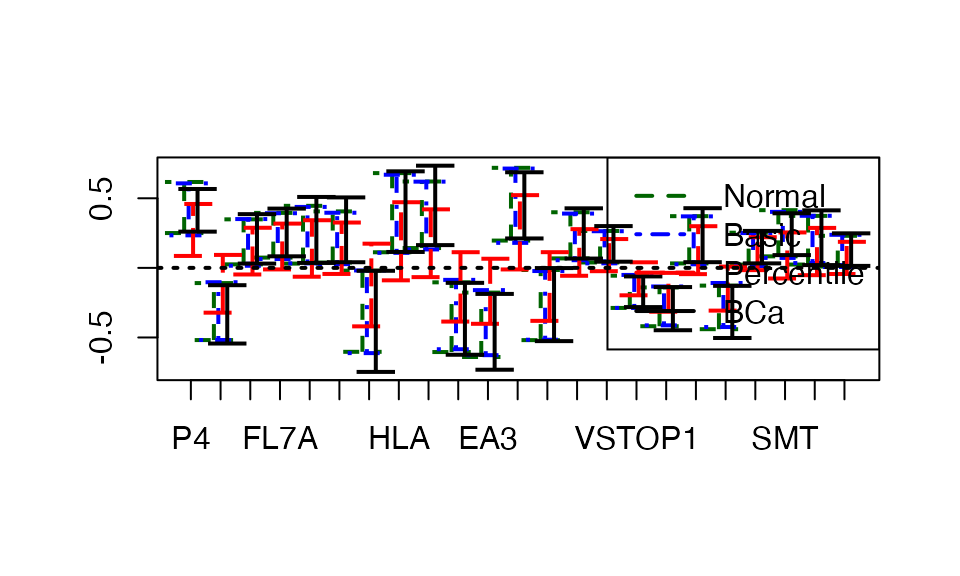
Figure 3. Bootstrap 95% confidence intervals, BCa significant variables, 6 components BR.
#TxTum <- read.table("MET_rev_edt.txt",sep="\t",header=TRUE)

data("TxTum.mod.bootBC1")

temp.ci <- plsRglm::confints.bootpls(TxTum.mod.bootBC1)

data("ind_BCa_nt1BC")
data("ind_BCa_nt2BC")
data("ind_BCa_nt3BC")
data("ind_BCa_nt4BC")
data("ind_BCa_nt5BC")
data("ind_BCa_nt6BC")
data("ind_BCa_nt1BR")
data("ind_BCa_nt2BR")
data("ind_BCa_nt3BR")
data("ind_BCa_nt4BR")
data("ind_BCa_nt5BR")
data("ind_BCa_nt6BR")

rownames(temp.ci)[ind_BCa_nt1BC]
#>  [1] "P4"     "E1"     "RB"     "P53"    "HLA"    "EA2"    "F3B"    "VSEGFR"
#>  [9] "SHL"    "SEB"
(colnames(TxTum.mod.bootBC1$data)[-1])[]
#>  [1] "age"      "sexe"     "HISTOADK" "H2"       "P3"       "P4"
#>  [7] "E1"       "P5"       "R10"      "C3M"      "P6"       "RB"
#> [13] "FL7A"     "P53"      "W2"       "P2"       "P1"       "W4"
#> [19] "MT1"      "MT2"      "MT4"      "MT3"      "HLA"      "HLD"
#> [25] "HLC"      "HLB"      "EA1"      "EA3"      "EA2"      "EA4"
#> [31] "EB1"      "EB2"      "EB3"      "EB4"      "EGF1"     "EGF2"
#> [37] "EGF3"     "EGF4"     "EGF5"     "EGF6"     "FL7B"     "VSFGF7"
#> [43] "F3A"      "F3B"      "VSFGFR3"  "F4"       "Q5"       "VSTOP1"
#> [49] "VSTOP2A"  "VSEGFR"   "AFRAEGFR" "SRXRA"    "SMT"      "QMTAMPN"
#> [55] "QMTDELN"  "SHL"      "SEA"      "SEB"      "QPCRFGF7"

indics <- cbind(ind_BCa_nt1BC,
ind_BCa_nt2BC,
ind_BCa_nt3BC,
ind_BCa_nt4BC,
ind_BCa_nt5BC,
ind_BCa_nt6BC,
ind_BCa_nt1BR,
ind_BCa_nt2BR,
ind_BCa_nt3BR,
ind_BCa_nt4BR,
ind_BCa_nt5BR,
ind_BCa_nt6BR)

nbpreds <- rbind(colSums(indics[,1:6]),colSums(indics[,7:12]))
colnames(nbpreds) <- c("1","2","3","4","5","6")
rownames(nbpreds) <- c("BC","BR")
nbpreds
#>     1 2  3  4  5  6
#> BC 10 7 11 15 23 24
#> BR  9 7  9 15 21 23
inone <- indics[rowSums(indics)>0,c(1,7,2,8,3,9,4,10,5,11,6,12)]
inone <- t(apply(inone,1,as.numeric))
rownames(inone)
#>  [1] "age"      "P4"       "E1"       "C3M"      "RB"       "FL7A"
#>  [7] "P53"      "W2"       "P2"       "W4"       "MT4"      "HLA"
#> [13] "HLD"      "HLB"      "EA3"      "EA2"      "EB4"      "EGF2"
#> [19] "EGF3"     "EGF4"     "FL7B"     "F3B"      "VSFGFR3"  "VSTOP1"
#> [25] "VSTOP2A"  "VSEGFR"   "AFRAEGFR" "SRXRA"    "SMT"      "SHL"
#> [31] "SEA"      "SEB"
colnames(inone) <- c("BC1","BR1","BC2","BR2","BC3","BR3","BC4","BR4","BC5","BR5","BC6","BR6")
colnames(inone) <- c("1 BC","  BR","2 BC","  BR","3 BC","  BR","4 BC","  BR","5 BC","  BR","6 BC","  BR")
inone
#>          1 BC   BR 2 BC   BR 3 BC   BR 4 BC   BR 5 BC   BR 6 BC   BR
#> age         0    0    0    0    0    0    1    1    0    0    0    0
#> P4          1    1    1    1    1    1    1    1    1    1    1    1
#> E1          1    1    1    1    1    1    1    1    0    0    0    0
#> C3M         0    0    0    0    0    0    1    1    1    1    1    1
#> RB          1    1    1    1    1    1    1    1    1    1    1    1
#> FL7A        0    0    1    1    1    0    1    1    1    1    1    1
#> P53         1    1    1    1    1    1    1    1    1    1    0    0
#> W2          0    0    0    0    0    0    0    0    1    1    1    1
#> P2          0    0    0    0    1    1    0    0    0    0    0    0
#> W4          0    0    0    0    0    0    1    1    1    1    1    1
#> MT4         0    0    0    0    0    0    0    0    1    0    1    1
#> HLA         1    0    0    0    1    1    1    1    1    1    1    1
#> HLD         0    0    0    0    1    1    1    1    1    1    1    1
#> HLB         0    0    0    0    0    0    0    0    1    1    1    1
#> EA3         0    0    0    0    0    0    0    0    1    1    1    1
#> EA2         1    1    1    1    1    1    1    1    1    1    1    1
#> EB4         0    1    0    0    0    0    0    0    0    0    0    0
#> EGF2        0    0    0    0    0    0    0    0    1    0    1    1
#> EGF3        0    0    0    0    0    0    0    0    0    0    1    0
#> EGF4        0    0    0    0    0    0    1    1    0    0    0    0
#> FL7B        0    0    0    0    0    0    0    0    1    1    1    1
#> F3B         1    1    0    0    0    0    0    0    0    0    0    0
#> VSFGFR3     0    0    0    0    0    0    0    0    1    1    1    1
#> VSTOP1      0    0    0    0    0    0    0    0    1    1    1    1
#> VSTOP2A     0    0    0    0    1    1    1    1    1    1    1    1
#> VSEGFR      1    1    0    0    0    0    1    1    1    1    1    1
#> AFRAEGFR    0    0    0    0    0    0    1    1    1    1    1    1
#> SRXRA       0    0    0    0    0    0    0    0    1    1    1    1
#> SMT         0    0    0    0    0    0    0    0    1    1    1    1
#> SHL         1    0    0    0    1    0    0    0    0    0    1    1
#> SEA         0    0    1    1    0    0    0    0    0    0    0    0
#> SEB         1    1    0    0    0    0    0    0    1    1    1    1
library(bipartite)
#> Loading required package: sna
#> Loading required package: statnet.common
#>
#> Attaching package: 'statnet.common'
#> The following objects are masked from 'package:base':
#>
#>     attr, order, replace
#> Loading required package: network
#>
#> 'network' 1.19.0 (2024-12-08), part of the Statnet Project
#> * 'news(package="network")' for changes since last version
#> * 'citation("network")' for citation information
#> * 'https://statnet.org' for help, support, and other information
#> sna: Tools for Social Network Analysis
#> Version 2.8 created on 2024-09-07.
#> copyright (c) 2005, Carter T. Butts, University of California-Irvine
#>  For citation information, type citation("sna").
#>  Type help(package="sna") to get started.
#> Loading required package: vegan
#> Loading required package: permute
#>  This is bipartite 2.22.
#>  For latest changes see versionlog in ?"bipartite-package". For citation see: citation("bipartite").
#>  Have a nice time plotting and analysing two-mode networks.
#>
#> Attaching package: 'bipartite'
#> The following object is masked from 'package:vegan':
#>
#>     nullmodel
bipartite::visweb(t(inone),type="None",labsize=2,square="b",box.col="grey25",pred.lablength=7)
Figure 4. Selected variables using the bootstrap BCa technique.
Example of application in chemometrics
The goal is to find compounds that can predict the rate of cancer cell infiltration in patients from spectrometry data. A healthy patient has 0 % of cancer cells in a biopsy while a sick patient will have in a biopsy a % higher than the sample contains cancer cells. The interest of this experiment is to try to reduce considerably the time of analysis of the biopsies by avoiding the need for a counting by a doctor specialized in anatomy and pathological cytology. An additional statistical difficulty appears here: there are more variables (180) than individuals (80). More details on the experimental protocol followed are available in the article in which this dataset has already been published (Piotto, 2012)41.
We begin by determining the number of components to use to fit a model with all areas of the spectrum as explanatory variables. Table 5 contains the components for selecting the number of components. We again see the tendency of the AIC and BIC criteria to retain a very high number of components, namely more than 10. On the other hand, in this example the criterion, estimated using a 10-group cross-validation (10-CV), seems relevant and invites us to keep 3 components. The same is true for the Pearson . The pseudo- is also in line with this since we observe a rapid decrease in the explanatory contribution following the addition of additional components beyond the third one.
| Nb of Comp. | 0 | 1 | 2 | 3 | 4 | 5 | 6 | 7 | 8 | 9 | 10 |
|---|---|---|---|---|---|---|---|---|---|---|---|
| AIC | |||||||||||
| BIC | |||||||||||
| (10-CV) | |||||||||||
| Pearson | |||||||||||
| pseudo- | |||||||||||
| Pearson |
We then construct bootstrap samples of size 250 of the predictor coefficients for a 3-component model with the bias reduction (BR) method. Figure 5 gives the whisker boxes of these distributions. Confidence intervals are then obtained for each of the predictors with the normal, basic, percentile or techniques. In the end, we use the technique, known for its good properties (Diciccio, 1996)42, to select the significant variables at the 5 % threshold by retaining those for which the confidence interval does not contain 0 as illustrated by Figure 6 for the case of the 3-component model with the BR bias reduction technique.
data(colon)
orig <- colon
modpls.boot3 <- bootplsbeta(plsRbeta(X..Cellules.tumorales~.,data=colon,nt=3,modele="pls-beta"), sim="ordinary", stype="i", R=250)
#save(modpls.boot3,file="modpls.boot_nt3.Rdata")
data("modpls.boot_nt3")
temp.ci <- suppressWarnings(plsRglm::confints.bootpls(modpls.boot3))
ind_BCa_nt3 <- (temp.ci[,7]<0&temp.ci[,8]<0)|(temp.ci[,7]>0&temp.ci[,8]>0)
#save(ind_BCa_nt3,file="ind_BCa_nt3.Rdata")
boxplots.bootpls(modpls.boot3,indices = 2:nrow(temp.ci))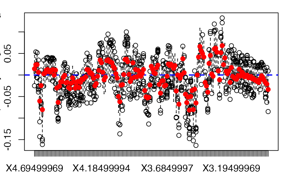
Figure 5. Boxplots of the bootstrap distribution of the coefficients of the predictors, 3 components BR
plsRglm::plots.confints.bootpls(temp.ci,prednames=TRUE,indices = 2:nrow(temp.ci))
Figure 6. Bootstrap 95% confidence intervals, 3 components BR
data(file="ind_BCa_nt3")
rownames(temp.ci)[ind_BCa_nt3]
#>  [1] "Intercept"   "X4.68499947" "X4.67499971" "X4.65499973" "X4.63499975"
#>  [6] "X4.52499962" "X4.51499987" "X4.50499964" "X4.45499992" "X4.43499947"
#> [11] "X4.42499971" "X4.41499949" "X4.38499975" "X4.37499952" "X4.35499954"
#> [16] "X4.23499966" "X4.2249999"  "X4.19499969" "X4.18499994" "X4.1449995"
#> [21] "X4.13499975" "X4.12499952" "X4.10499954" "X4.05499983" "X4.0449996"
#> [26] "X4.00499964" "X3.99499965" "X3.98499966" "X3.94499969" "X3.85499978"
#> [31] "X3.84499979" "X3.8349998"  "X3.82499981" "X3.80499983" "X3.75499964"
#> [36] "X3.73499966" "X3.67499971" "X3.65499973" "X3.64499974" "X3.59499979"
#> [41] "X3.56499982" "X3.54499984" "X3.53499961" "X3.52499962" "X3.51499963"
#> [46] "X3.50499964" "X3.49499965" "X3.48499966" "X3.46499968" "X3.44499969"
#> [51] "X3.4349997"  "X3.42499971" "X3.41499972" "X3.40499973" "X3.39499974"
#> [56] "X3.38499975" "X3.37499976" "X3.36499977" "X3.35499978" "X3.32499981"
#> [61] "X3.31499982" "X3.30499983" "X3.27499962" "X3.26499963" "X3.24499965"
#> [66] "X2.92499971" "X2.91499972"
plsRglm::plots.confints.bootpls(temp.ci,prednames=TRUE,indices = (2:nrow(temp.ci))[ind_BCa_nt3[-1]],articlestyle=FALSE)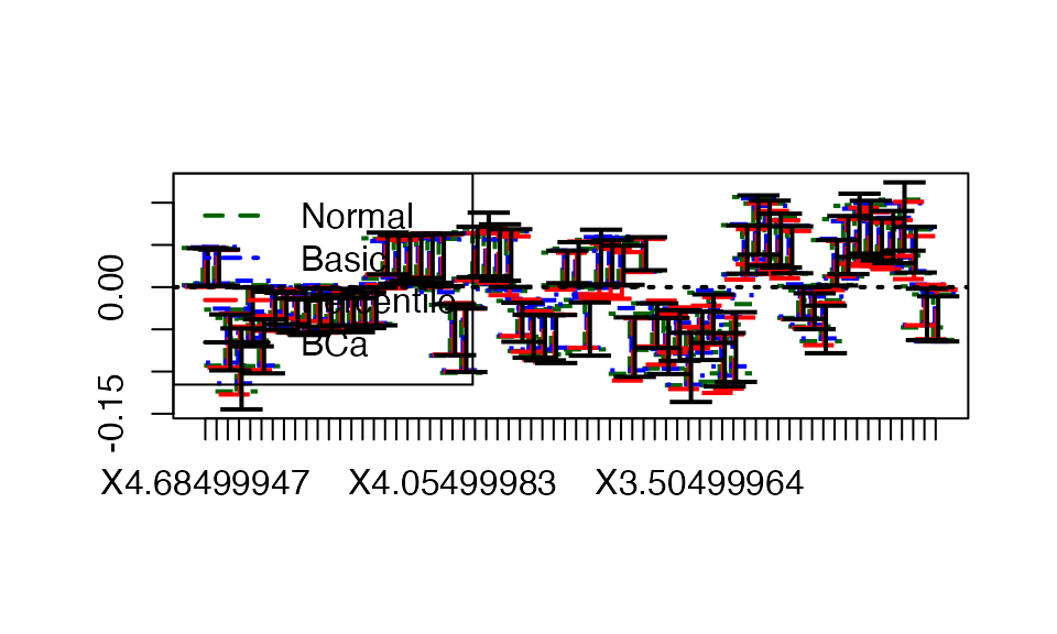
Figure 7. Bootstrap 95% confidence intervals, BCa significant variables, 3 components BR.
plsRglm::plots.confints.bootpls(temp.ci,prednames=TRUE,indices = (2:nrow(temp.ci))[ind_BCa_nt3[-1]],articlestyle=FALSE,typeIC="BCa")
Figure 8. BCa Bootstrap 95% confidence intervals, BCa significant variables, 3 components BR.
Finally, we fit a Beta PLS regression model constructed from the only 79 significant predictors for the bootstrap technique. The selection of the number of components, not reproduced here due to lack of space, leads us to retain 2 of them.
modpls_sub4 <- plsRbeta(X..Cellules.tumorales~.,data=colon_sub4,nt=10,modele="pls-beta")
#save(modpls_sub4,file="modpls_sub4.Rdata")
data("modpls_sub4")
modpls_sub4
#> Number of required components:
#> [1] 10
#> Number of successfully computed components:
#> [1] 10
#> Coefficients:
#>                     [,1]
#> Intercept      1.5448748
#> X4.65499973   61.1773419
#> X4.6449995   306.0463140
#> X4.63499975 -284.4099752
#> X4.60499954  130.5717258
#> X4.59499979   20.9463141
#> X4.58499956 -281.2770768
#> X4.57499981 -144.3983544
#> X4.56499958  641.2859589
#> X4.55499983  942.5579964
#> X4.52499962   72.6143880
#> X4.51499987 -251.4256475
#> X4.50499964  -10.2039878
#> X4.43499947 -138.0766836
#> X4.42499971 -880.1560188
#> X4.38499975 -941.1056739
#> X4.37499952 -784.5708620
#> X4.35499954  -68.8364717
#> X4.2949996   109.1380862
#> X4.28499985  289.5456254
#> X4.27499962 -322.5710004
#> X4.26499987   71.6963047
#> X4.25499964  304.2135548
#> X4.20499992  481.8986709
#> X4.19499969  663.7076930
#> X4.18499994   79.9407749
#> X4.1449995   -27.1338795
#> X4.13499975   -0.6603306
#> X4.12499952    5.0923295
#> X4.11499977   -6.9928171
#> X4.10499954    7.3648246
#> X4.09499979   86.6345576
#> X4.05499983  -20.4373561
#> X4.0449996  -132.2956632
#> X4.00499964   -0.6487794
#> X3.99499965  -28.7700528
#> X3.98499966  -11.1008973
#> X3.85499978  201.1209855
#> X3.84499979 -112.9491585
#> X3.8349998  -112.0879668
#> X3.82499981 -176.4575677
#> X3.81499982 -499.4286464
#> X3.80499983   96.0999755
#> X3.7949996  -130.6062827
#> X3.76499963    2.2957805
#> X3.75499964   73.7212553
#> X3.73499966  110.5824104
#> X3.70499969   -9.6116865
#> X3.69499969    6.8740870
#> X3.66499972   -0.9445308
#> X3.65499973    7.7458993
#> X3.61499977    7.1671863
#> X3.59499979  -73.7235407
#> X3.56499982  -37.2007473
#> X3.54499984   27.1867459
#> X3.53499961    9.9491250
#> X3.52499962   -1.4676426
#> X3.51499963 -185.4622429
#> X3.50499964  201.8383573
#> X3.49499965 -390.4445054
#> X3.48499966 -141.9592003
#> X3.47499967 -134.0444094
#> X3.46499968 -141.0216380
#> X3.44499969  227.1789740
#> X3.4349997    -4.7983899
#> X3.42499971  -79.9664654
#> X3.41499972   26.0378859
#> X3.40499973    7.7258949
#> X3.37499976 -628.0508174
#> X3.36499977 -505.0750367
#> X3.35499978  140.4448861
#> X3.32499981  259.3811778
#> X3.31499982 -276.7503657
#> X3.30499983  491.7257390
#> X3.27499962   37.4180261
#> X3.26499963   28.6326050
#> X3.25499964   16.3911723
#> X3.24499965   37.8061066
#> X3.19499969  -32.7055621
#> X3.13499975  256.5034605
#> Information criteria and Fit statistics:
#>                   AIC        BIC Chi2_Pearson_Y     RSS_Y pseudo_R2_Y      R2_Y
#> Nb_Comp_0   -32.34558  -27.58152       76.77937 6.4449550          NA        NA
#> Nb_Comp_1  -129.57972 -122.43364       79.47275 2.2942689   0.7755421 0.6440210
#> Nb_Comp_2  -134.63789 -125.10979       72.20098 1.9728198   0.7991522 0.6938970
#> Nb_Comp_3  -142.69157 -130.78143       79.01884 1.8772302   0.8279202 0.7087287
#> Nb_Comp_4  -155.51742 -141.22526       84.08689 1.5340918   0.8558543 0.7619701
#> Nb_Comp_5  -164.67721 -148.00302       79.11247 1.3100325   0.8743807 0.7967352
#> Nb_Comp_6  -169.31896 -150.26274       75.81459 1.1376671   0.8794340 0.8234794
#> Nb_Comp_7  -171.85756 -150.41932       75.94769 1.1110661   0.8924862 0.8276068
#> Nb_Comp_8  -176.91620 -153.09593       71.83334 0.9526869   0.8974669 0.8521810
#> Nb_Comp_9  -186.16095 -159.95866       72.24187 0.8050430   0.9039681 0.8750894
#> Nb_Comp_10 -190.25562 -161.67130       71.24851 0.7212852   0.9063458 0.8880853
# Index plot
sfit <- modpls_sub4$FinalModel;
rd <- resid(sfit, type="sweighted2");
plot(seq(1,sfit$n), rd, xlab="Subject Index", ylab="Std Weigthed Resid 2",
     main="Index Plot");
abline(h=0, lty=3);
Figure 9. Residuals index plot.
We note on Figure 10 that this model is validated by the use of a simulated envelope (Atkinson, 1981)43. This one is constructed, as recommended by Atkinson, from 19 order statistics.
library(betareg)
# A Half-normal Plot with simulated envelop
phat <- predict(sfit, type="response");
phihat <- predict(sfit, type="precision");
tt <- modpls_sub4$tt
n <- sfit$n
absrds <- list();
for (i in 1:19)
  {
     tYwotNA <- rbeta(sfit$n, phat*phihat, (1-phat)*phihat);
     tsfit <- betareg(tYwotNA~tt, x=TRUE);
     trd <- residuals(tsfit, type="sweighted2");
     absrds[[i]]<-sort(abs(trd));
  }
lower <- upper <- middle <- rep(0, n);
for (j in 1:n) {
   min <- max <- sum <- absrds[[1]][j];
   min; max;
   for (i in 2:19) {
      if (min > absrds[[i]][j]) min <- absrds[[i]][j];
      if (max < absrds[[i]][j]) max <- absrds[[i]][j];
      sum <- sum + absrds[[i]][j];
   }
   lower[j] <- min;
   upper[j] <- max;
   middle[j] <- sum / 19;
}

qnval <- qnorm((1:n+n-1/8) / (2*n+1/2));
plot(qnval, sort(abs(rd)), ylim=range(0,3.5), xlab="Expected", ylab="Observed",
     main="Half-Normal Plot with Simulated Envelope");
lines(qnval, lower, lty=3);
lines(qnval, upper, lty=3);
lines(qnval, middle, lty=1, lwd=2);
Figure 10. Residuals and simulated envelop.
As we can see in Figure 11, the two components of the model formed by the only 79 significant predictors for the bootstrap technique allow a clear linear separation between the healthy subjects, in dark green, and the sick subjects whose condition is all the more serious as the color approaches red. To allow a graphical evaluation of the predictive quality of the model, we represent the observed values as a function of the predicted values on the scale, Figure 12, and on the original scale Figure 13. Note that, since the transition from one to the other of the two graphs is done by means of a continuous, bijective and increasing transformation of the axes, the Kendall correlation coefficient between the observed and predicted values will be identical for both scales. For both graphs, we measure an association in the sense of Kendall’s correlation coefficient between the observed values and the predicted values equal to for a -value of , thus significant at the threshold.
plot(modpls_sub4$tt[,1],modpls_sub4$tt[,2],col=plotrix::color.scale(colon[,1],c(0,1,1),c(1,1,0),0),pch=16,ylab="",xlab="")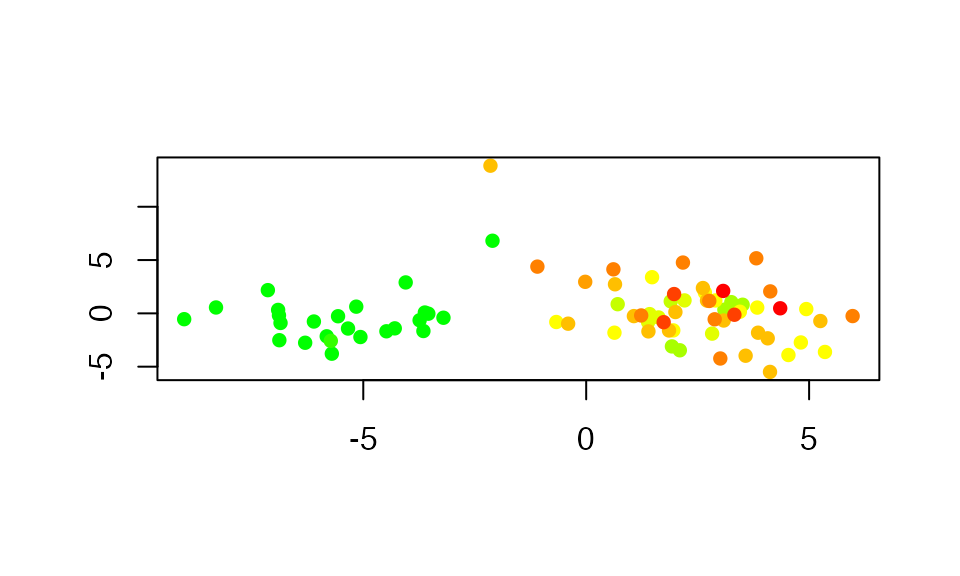
Figure 11. Representation of individuals on the plane formed by the first two components.
plot(binomial()$linkfun(modpls_sub4$ValsPredictY),binomial()$linkfun(orig[,1]),xlab="Valeurs prédites",ylab="Valeurs observées")
abline(0,1,lwd=2,lty=2)
Figure 12. Observed values versus predicted values on the logit scale.

Figure 13. Observed values versus predicted values on the original scale.
Note, however, that the data in this example are in fact formed by mixing healthy individuals for whom the infiltration rate is zero and sick individuals for whom these rates are non-zero and vary from 0 to 1. Thus the use of a PLS regression model based on the combination of a logistic PLS regression model and a Beta logistic regression model or a Beta regression model with inflation of 0 introduced by Ospina and Ferrari (Ospina, 2012)44 would likely make sense and is currently being carried out by the authors.
Conclusion and perspectives
Our goal has been to propose an extension of PLS regression to Beta
regression models, and then to make it available to users of the free
language R.
We thus offer the possibility to work with collinear predictors to model rates or proportions, which is an unavoidable difficulty when modeling mixtures or when analyzing spectra or studying genetic, proteomic or metabonomic data.
Moreover, Beta PLS regression can also be applied to incomplete data sets. It is also possible in this case, as in the case of complete data, to select the number of components by repeated -fold cross-validation.
Finally, we propose bootstrap techniques in order to, for example, test the significance of each of the predictors present in the dataset and thus validate the models built.
The study of two real datasets allowed the proposed tools to demonstrate their efficiency.