Plot bootstrap confidence intervals

This function plots the confidence intervals derived using the function confints.bootpls from from a bootpls based object.

Usage

plots.confints.bootpls(
  ic_bootobject,
  indices = NULL,
  legendpos = "topleft",
  prednames = TRUE,
  articlestyle = TRUE,
  xaxisticks = TRUE,
  ltyIC = c(2, 4, 5, 1),
  colIC = c("darkgreen", "blue", "red", "black"),
  typeIC,
  las = par("las"),
  mar,
  mgp,
  ...
)

Arguments

ic_bootobject: an object created with the confints.bootpls function.
indices: vector of indices of the variables to plot. Defaults to NULL: all the predictors will be used.
legendpos: position of the legend as in legend, defaults to "topleft"
prednames: do the original names of the predictors shall be plotted ? Defaults to TRUE: the names are plotted.
articlestyle: do the extra blank zones of the margin shall be removed from the plot ? Defaults to TRUE: the margins are removed.
xaxisticks: do ticks for the x axis shall be plotted ? Defaults to TRUE: the ticks are plotted.
ltyIC: lty as in plot
colIC: col as in plot
typeIC: type of CI to plot. Defaults to typeIC=c("Normal", "Basic", "Percentile", "BCa") if BCa intervals limits were computed and to typeIC=c("Normal", "Basic", "Percentile") otherwise.
las: numeric in 0,1,2,3; the style of axis labels. 0: always parallel to the axis [default], 1: always horizontal, 2: always perpendicular to the axis, 3: always vertical.
mar: A numerical vector of the form c(bottom, left, top, right) which gives the number of lines of margin to be specified on the four sides of the plot. The default is c(5, 4, 4, 2) + 0.1.
mgp: The margin line (in mex units) for the axis title, axis labels and axis line. Note that mgp[1] affects title whereas mgp[2:3] affect axis. The default is c(3, 1, 0).
...: further options to pass to the plot function.

Value

NULL

Author

Frédéric Bertrand
frederic.bertrand@lecnam.net
https://fbertran.github.io/homepage/

Examples


data(Cornell)
modpls <- plsR(Y~.,data=Cornell,3)
#> ____************************************************____
#> ____Component____ 1 ____
#> ____Component____ 2 ____
#> ____Component____ 3 ____
#> ____Predicting X without NA neither in X nor in Y____
#> ****________________________________________________****
#> 

# Lazraq-Cleroux PLS (Y,X) bootstrap
set.seed(250)
Cornell.bootYX <- bootpls(modpls, R=250, verbose=FALSE)
temp.ci <- confints.bootpls(Cornell.bootYX,2:8)
#> Warning: extreme order statistics used as endpoints
#> Warning: extreme order statistics used as endpoints
#> Warning: extreme order statistics used as endpoints

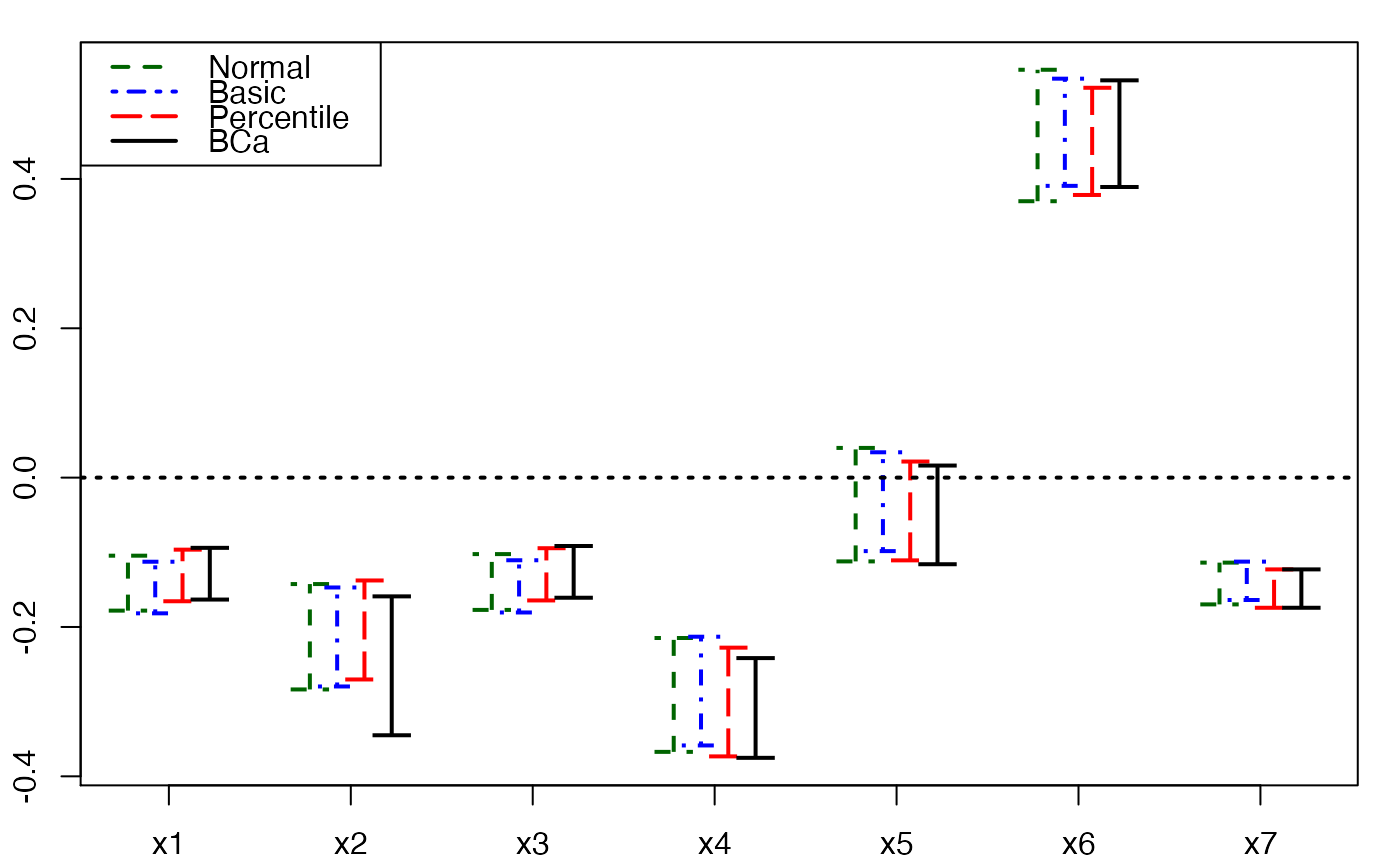
plots.confints.bootpls(temp.ci)

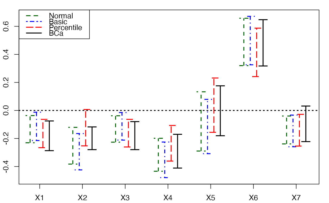plots.confints.bootpls(temp.ci,prednames=FALSE)

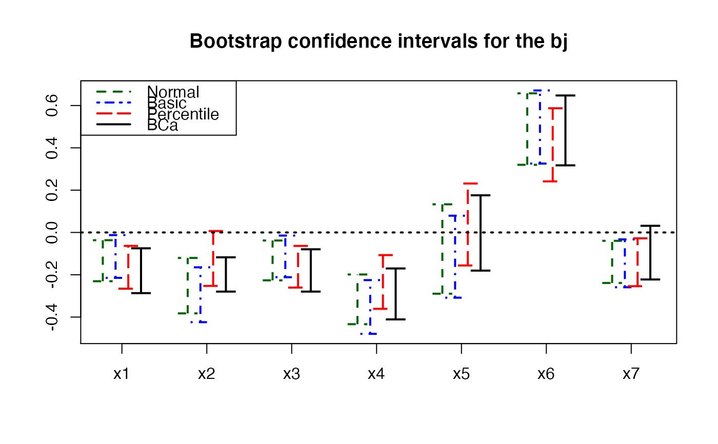
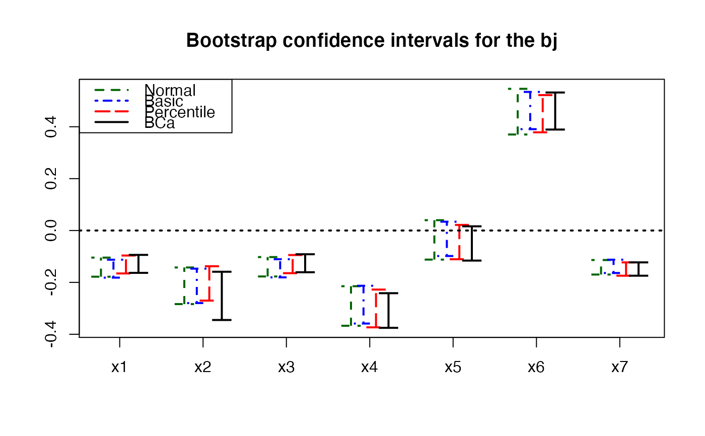
plots.confints.bootpls(temp.ci,prednames=FALSE,articlestyle=FALSE,
main="Bootstrap confidence intervals for the bj")

plots.confints.bootpls(temp.ci,indices=1:3,prednames=FALSE)

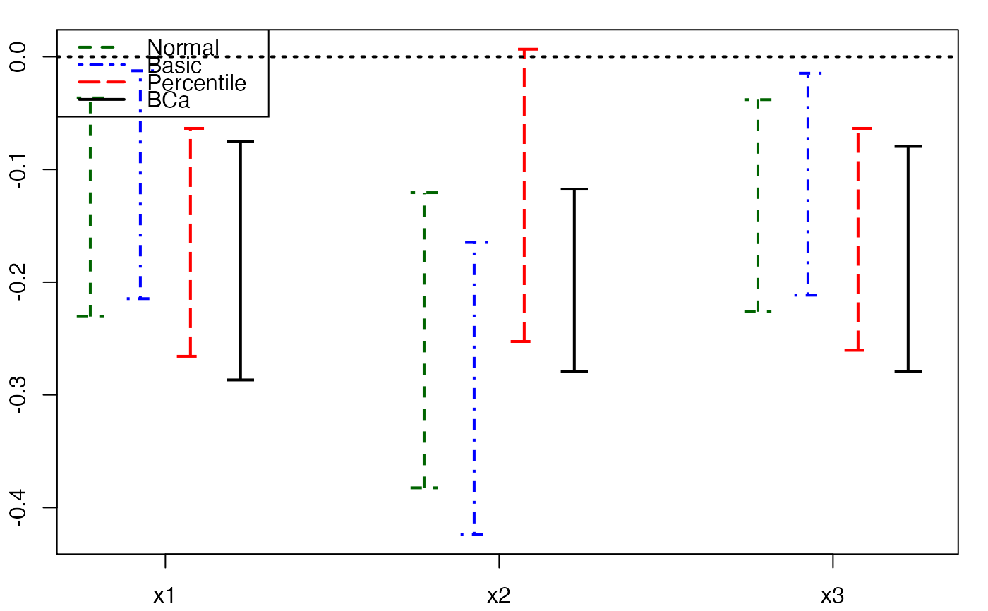
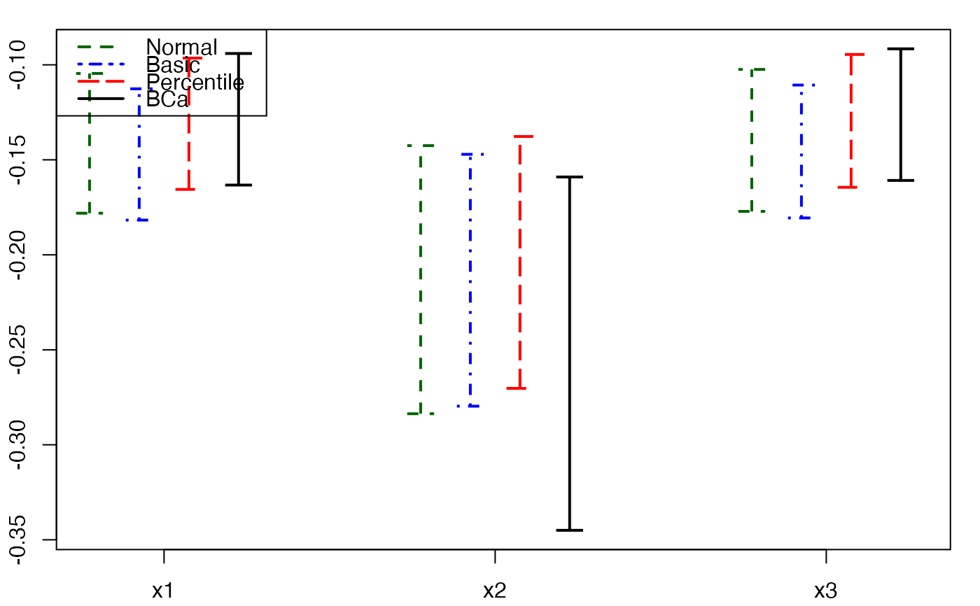
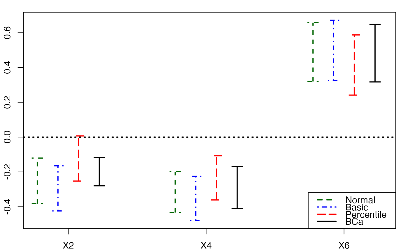
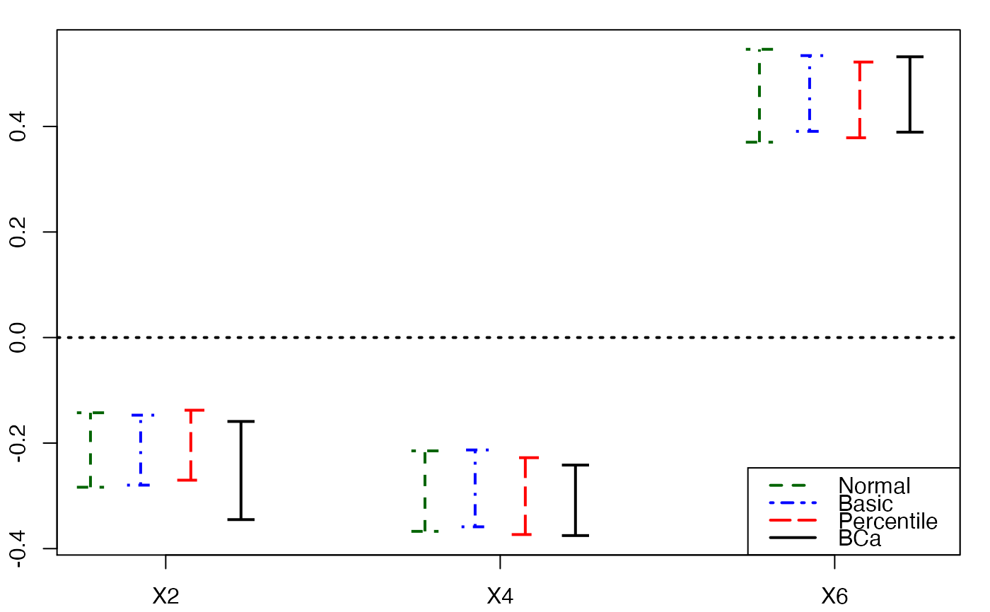
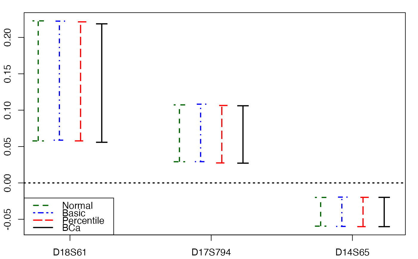
plots.confints.bootpls(temp.ci,c(2,4,6),"bottomright")

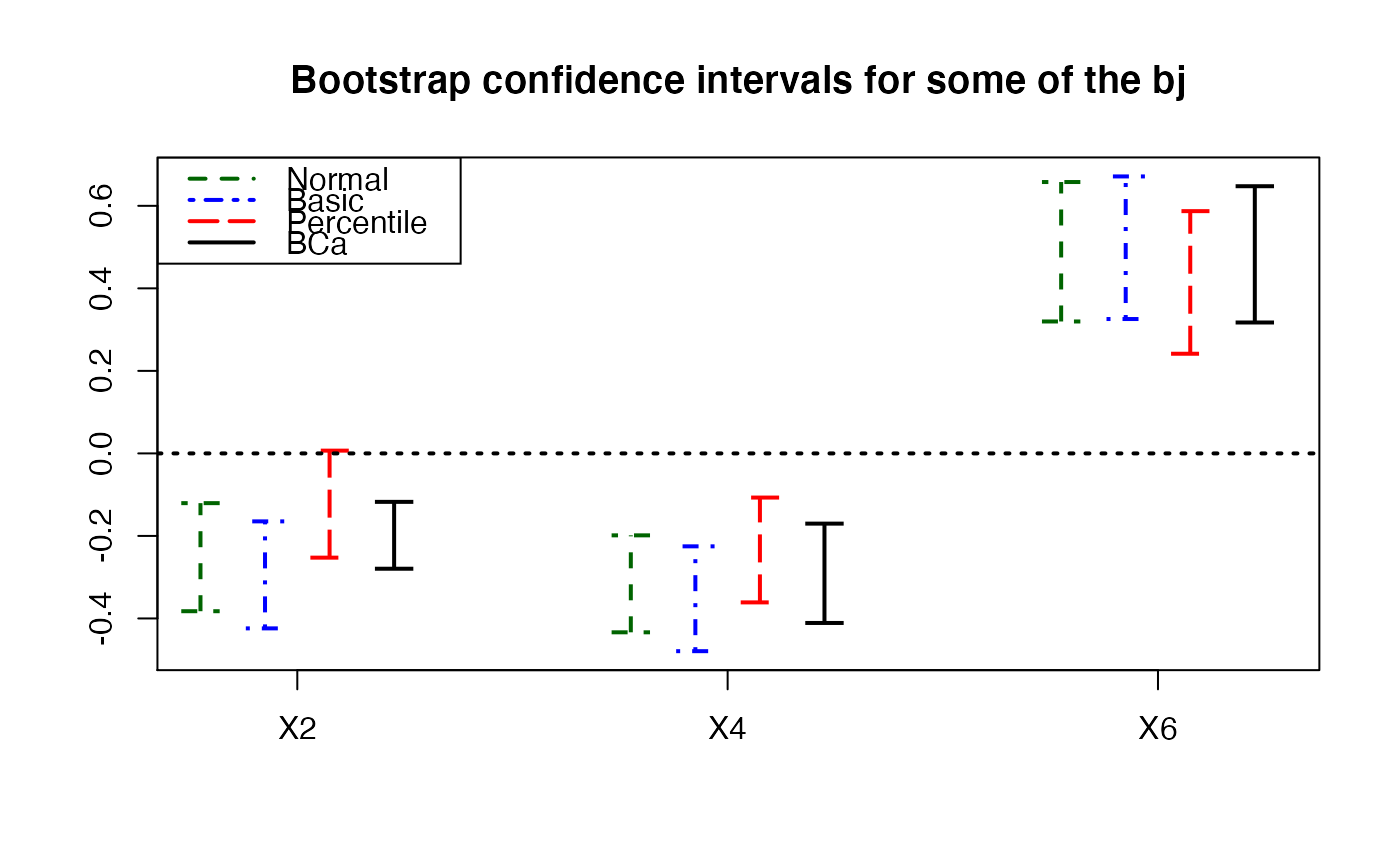
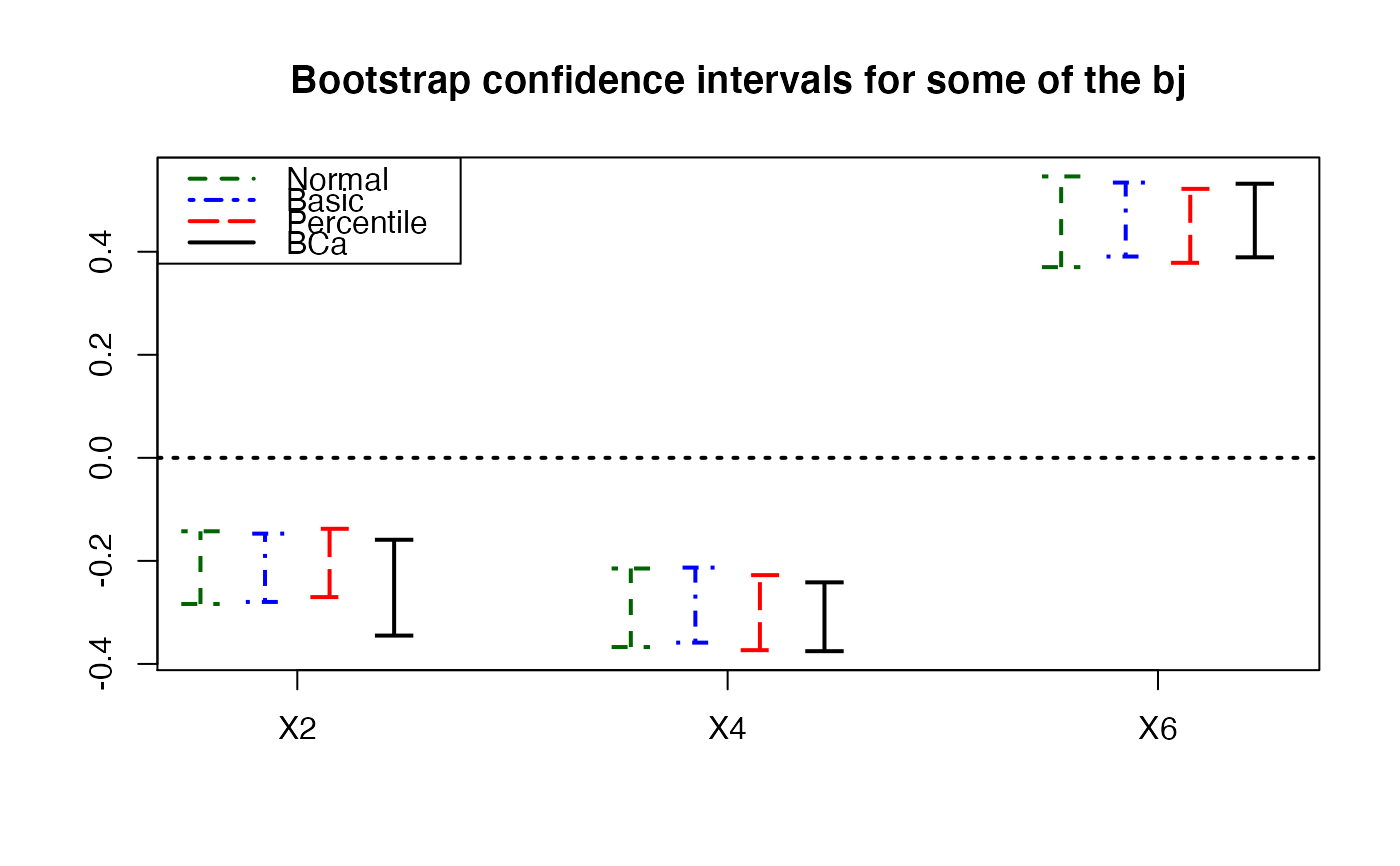
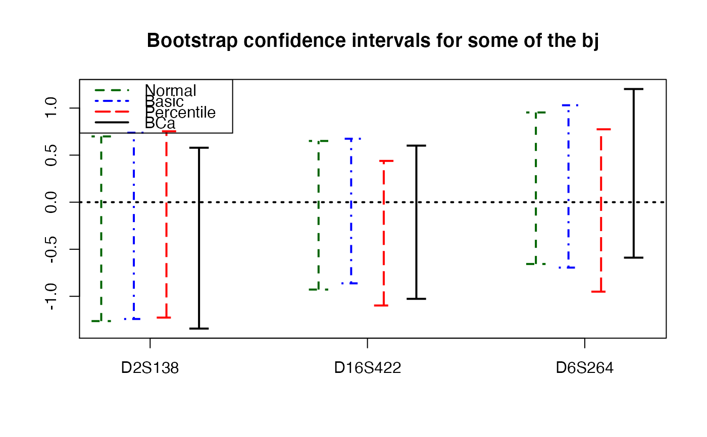
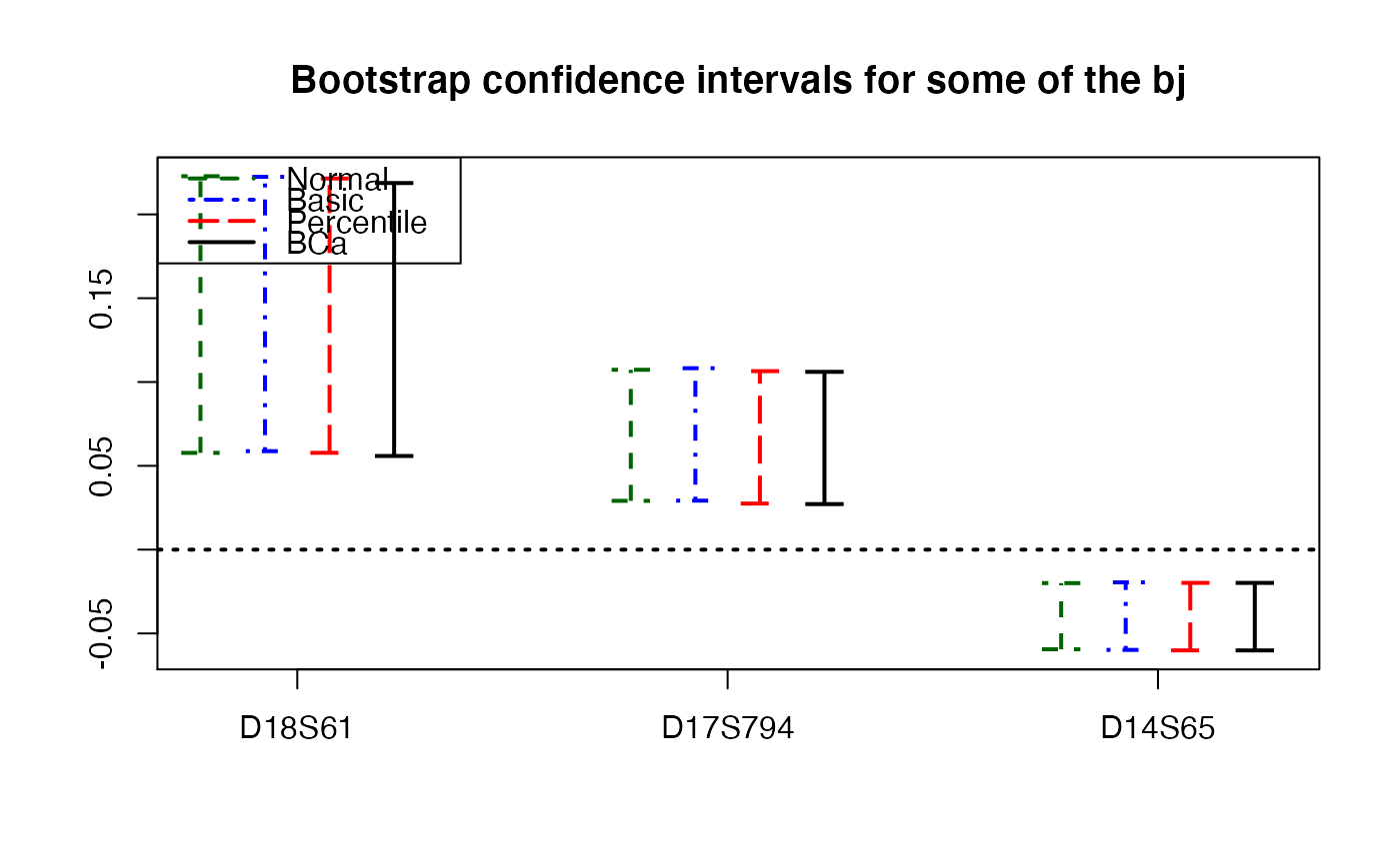
plots.confints.bootpls(temp.ci,c(2,4,6),articlestyle=FALSE,
main="Bootstrap confidence intervals for some of the bj")


temp.ci <- confints.bootpls(Cornell.bootYX,typeBCa=FALSE)
plots.confints.bootpls(temp.ci)
#> Warning: zero-length arrow is of indeterminate angle and so skipped
#> Warning: zero-length arrow is of indeterminate angle and so skipped
#> Warning: zero-length arrow is of indeterminate angle and so skipped

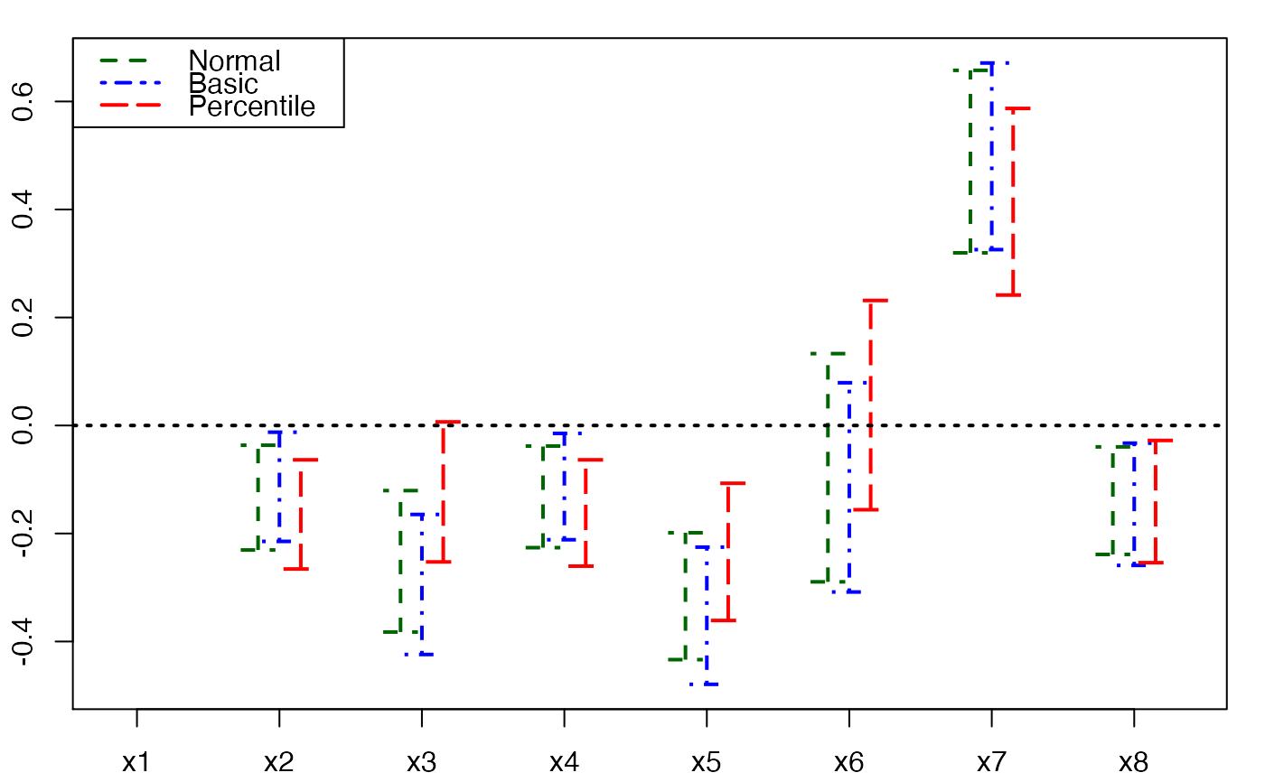
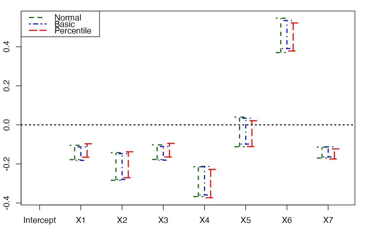
plots.confints.bootpls(temp.ci,2:8)

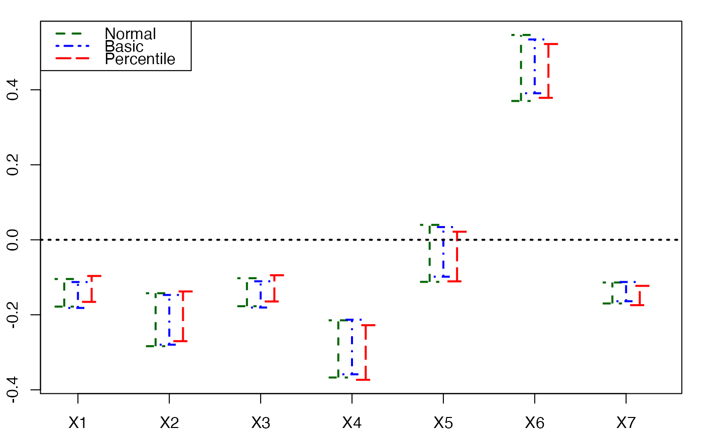
plots.confints.bootpls(temp.ci,prednames=FALSE)
#> Warning: zero-length arrow is of indeterminate angle and so skipped
#> Warning: zero-length arrow is of indeterminate angle and so skipped
#> Warning: zero-length arrow is of indeterminate angle and so skipped



# Bastien CSDA 2005 (Y,T) bootstrap
Cornell.boot <- bootpls(modpls, typeboot="fmodel_np", R=250, verbose=FALSE)
temp.ci <- confints.bootpls(Cornell.boot,2:8)

plots.confints.bootpls(temp.ci)

plots.confints.bootpls(temp.ci,prednames=FALSE)

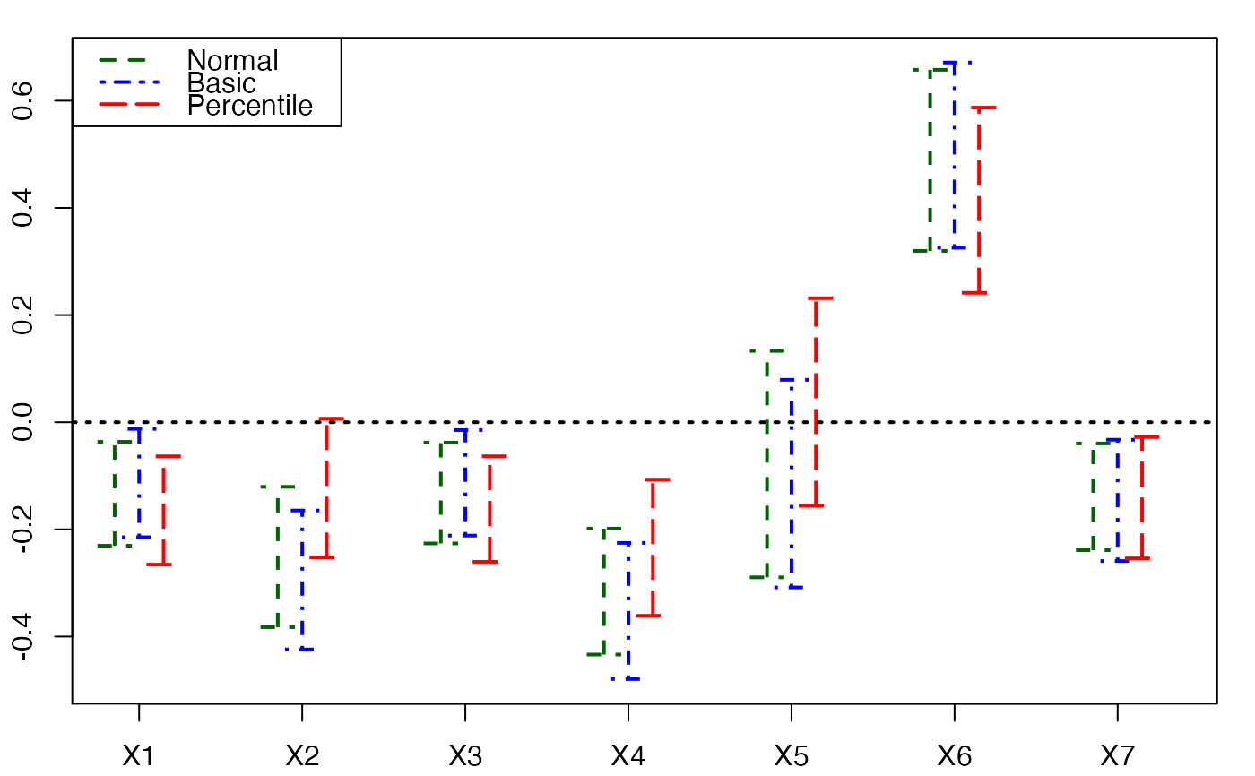
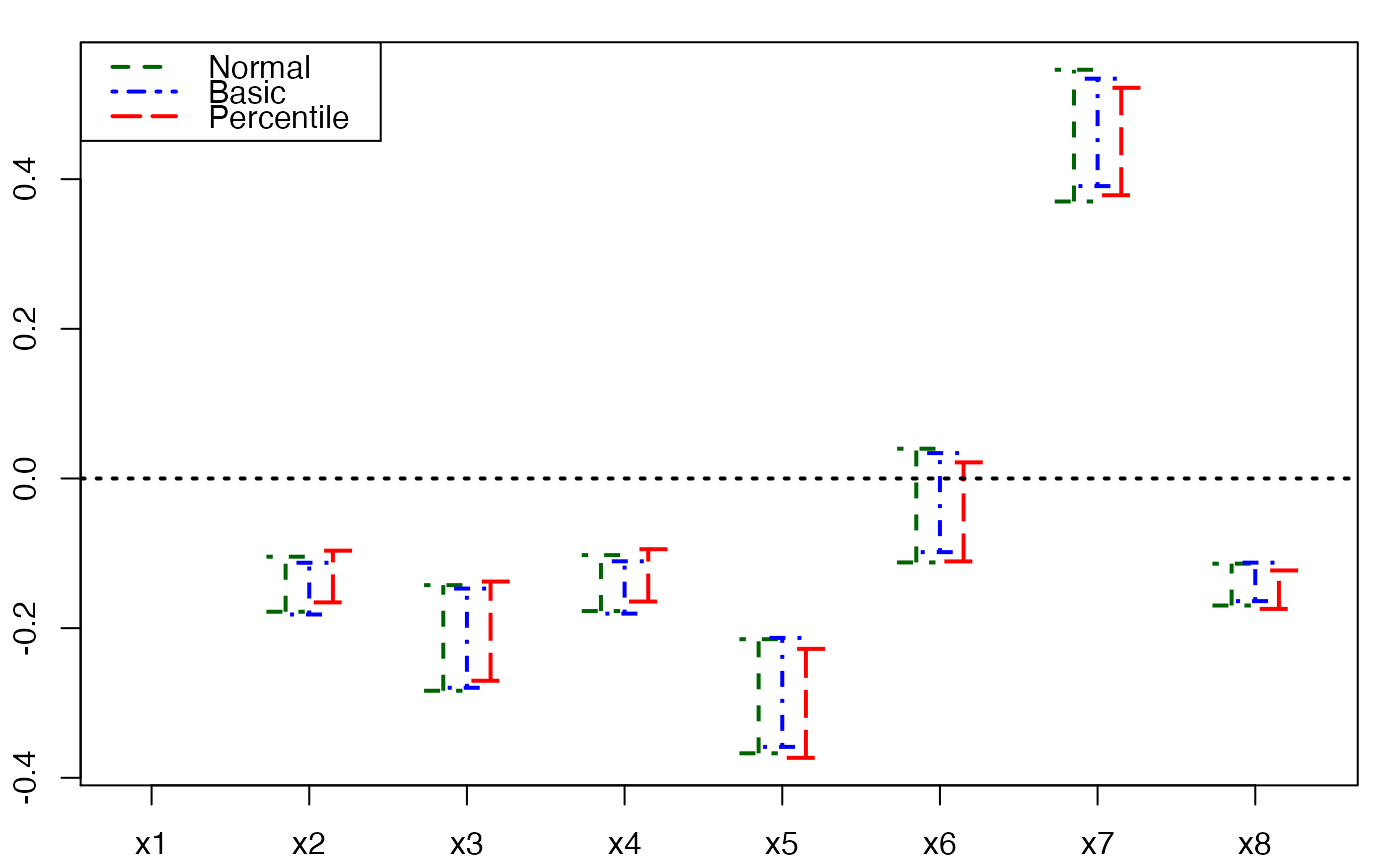
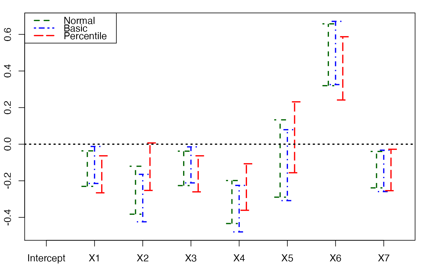
plots.confints.bootpls(temp.ci,prednames=FALSE,articlestyle=FALSE,
main="Bootstrap confidence intervals for the bj")

plots.confints.bootpls(temp.ci,indices=1:3,prednames=FALSE)

plots.confints.bootpls(temp.ci,c(2,4,6),"bottomright")

plots.confints.bootpls(temp.ci,c(2,4,6),articlestyle=FALSE,
main="Bootstrap confidence intervals for some of the bj")


temp.ci <- confints.bootpls(Cornell.boot,typeBCa=FALSE)
plots.confints.bootpls(temp.ci)
#> Warning: zero-length arrow is of indeterminate angle and so skipped
#> Warning: zero-length arrow is of indeterminate angle and so skipped
#> Warning: zero-length arrow is of indeterminate angle and so skipped

plots.confints.bootpls(temp.ci,2:8)

plots.confints.bootpls(temp.ci,prednames=FALSE)
#> Warning: zero-length arrow is of indeterminate angle and so skipped
#> Warning: zero-length arrow is of indeterminate angle and so skipped
#> Warning: zero-length arrow is of indeterminate angle and so skipped



# \donttest{
data(aze_compl)
modplsglm <- plsRglm(y~.,data=aze_compl,3,modele="pls-glm-logistic")
#> ____************************************************____
#> 
#> Family: binomial 
#> Link function: logit 
#> 
#> ____Component____ 1 ____
#> ____Component____ 2 ____
#> ____Component____ 3 ____
#> ____Predicting X without NA neither in X or Y____
#> ****________________________________________________****
#> 

# Lazraq-Cleroux PLS (Y,X) bootstrap
# should be run with R=1000 but takes much longer time
aze_compl.bootYX3 <- bootplsglm(modplsglm, typeboot="plsmodel", R=250, verbose=FALSE)
#> Warning: glm.fit: fitted probabilities numerically 0 or 1 occurred
#> Warning: glm.fit: fitted probabilities numerically 0 or 1 occurred
#> Warning: glm.fit: fitted probabilities numerically 0 or 1 occurred
#> Warning: glm.fit: fitted probabilities numerically 0 or 1 occurred
temp.ci <- confints.bootpls(aze_compl.bootYX3)
#> Warning: extreme order statistics used as endpoints
#> Warning: extreme order statistics used as endpoints
#> Warning: extreme order statistics used as endpoints
#> Warning: extreme order statistics used as endpoints
#> Warning: extreme order statistics used as endpoints
#> Warning: extreme order statistics used as endpoints

plots.confints.bootpls(temp.ci)

plots.confints.bootpls(temp.ci,prednames=FALSE)

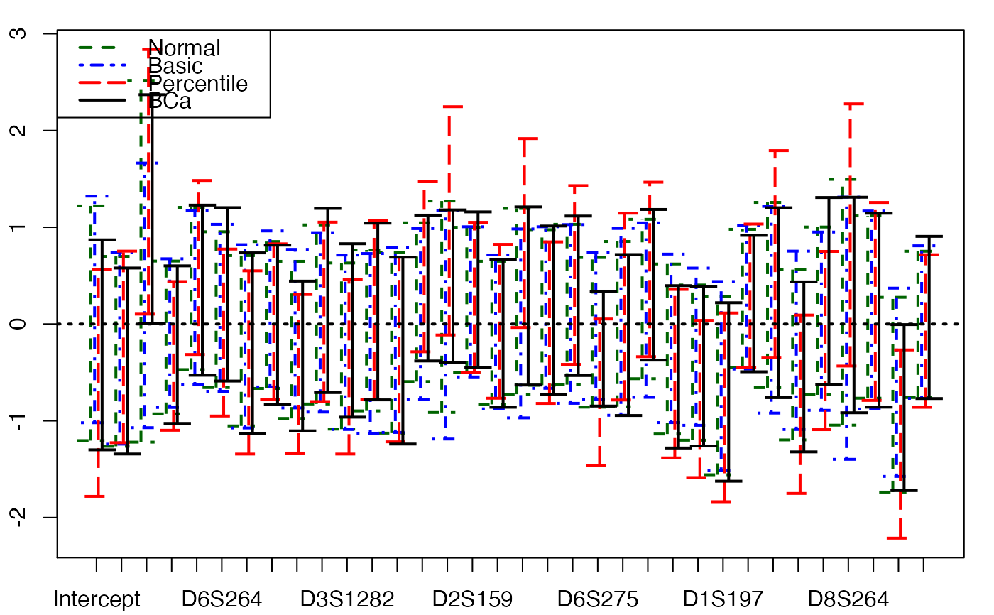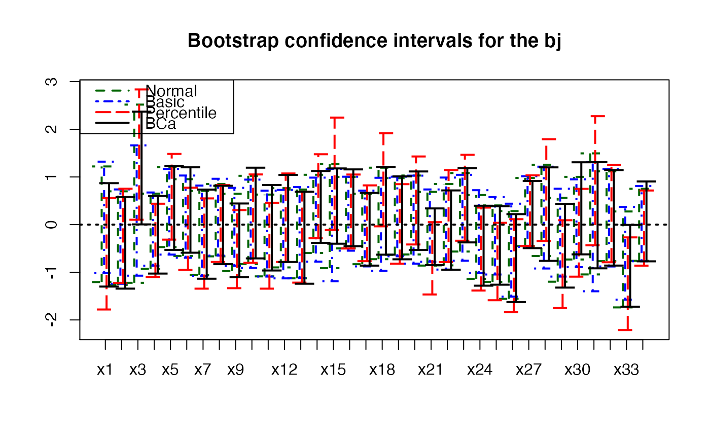
plots.confints.bootpls(temp.ci,prednames=FALSE,articlestyle=FALSE,
main="Bootstrap confidence intervals for the bj")

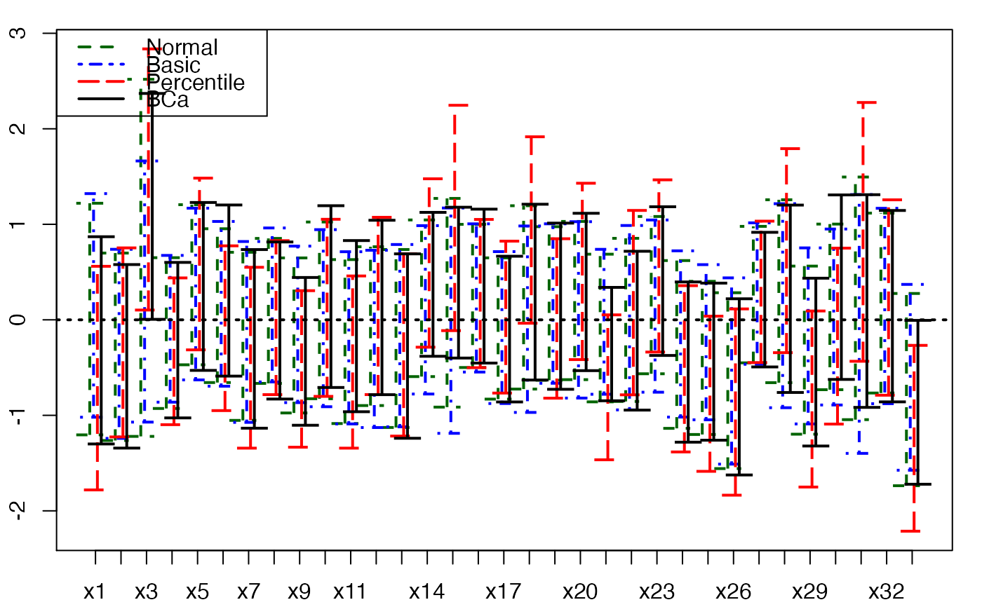
plots.confints.bootpls(temp.ci,indices=1:33,prednames=FALSE)

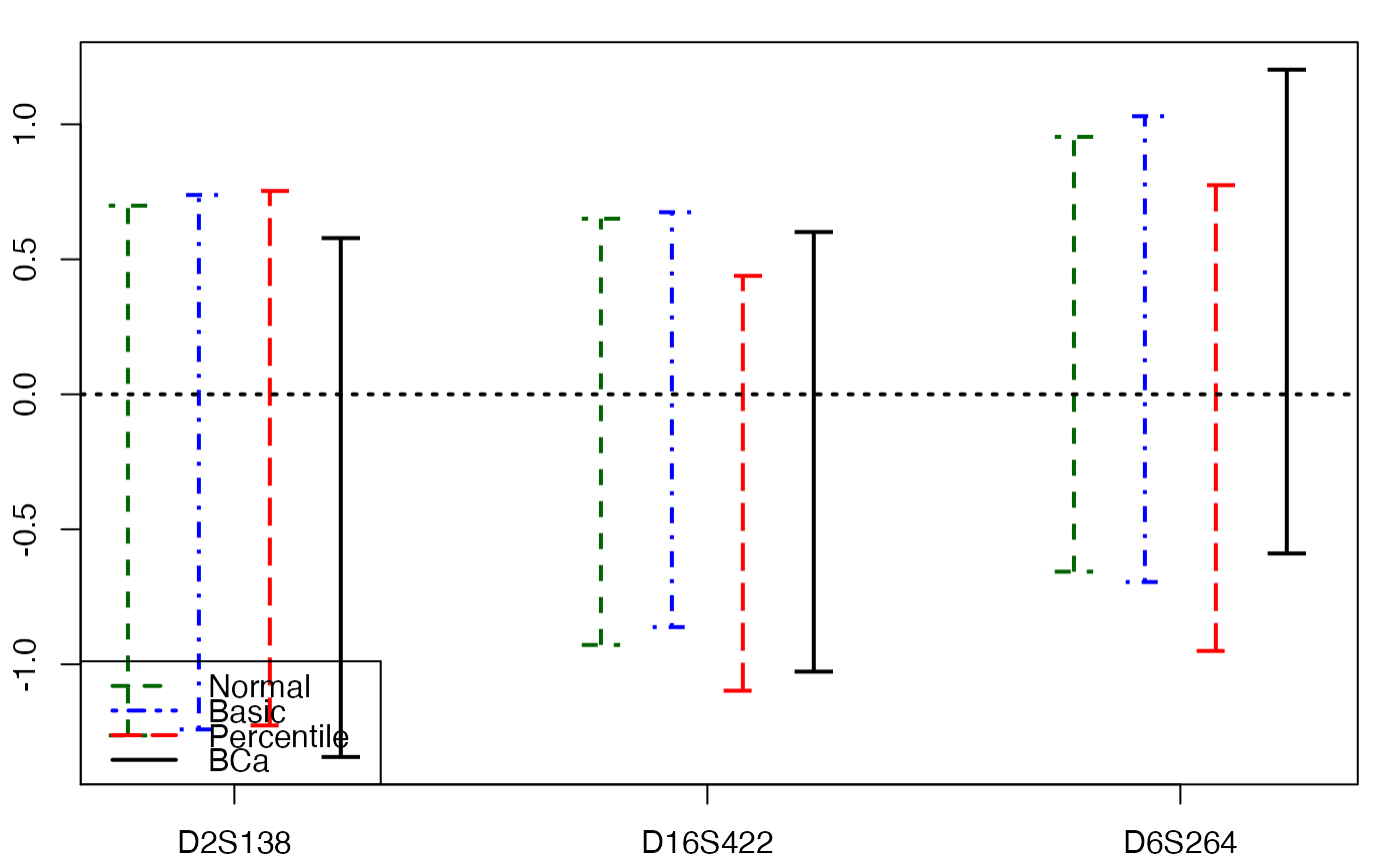
plots.confints.bootpls(temp.ci,c(2,4,6),"bottomleft")

plots.confints.bootpls(temp.ci,c(2,4,6),articlestyle=FALSE,
main="Bootstrap confidence intervals for some of the bj")

plots.confints.bootpls(temp.ci,indices=1:34,prednames=FALSE)

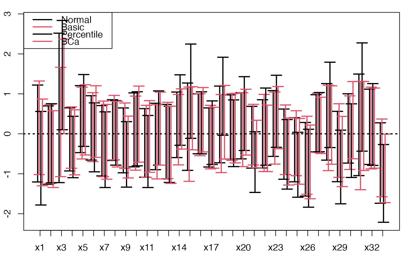
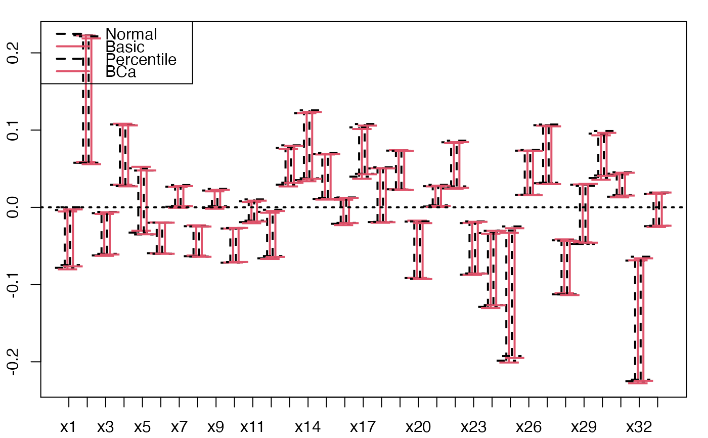
plots.confints.bootpls(temp.ci,indices=1:33,prednames=FALSE,ltyIC=1,colIC=c(1,2))

 
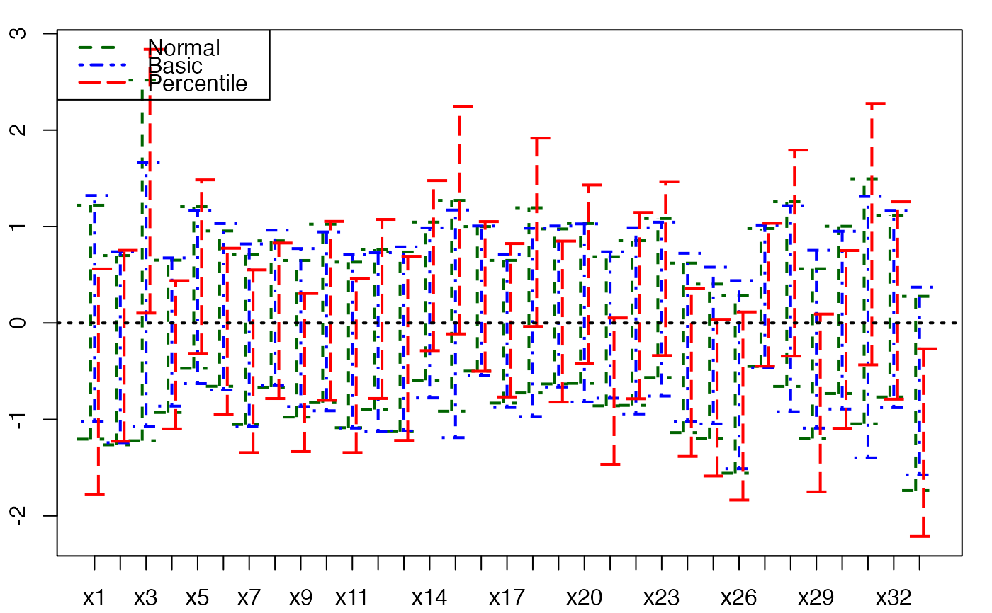
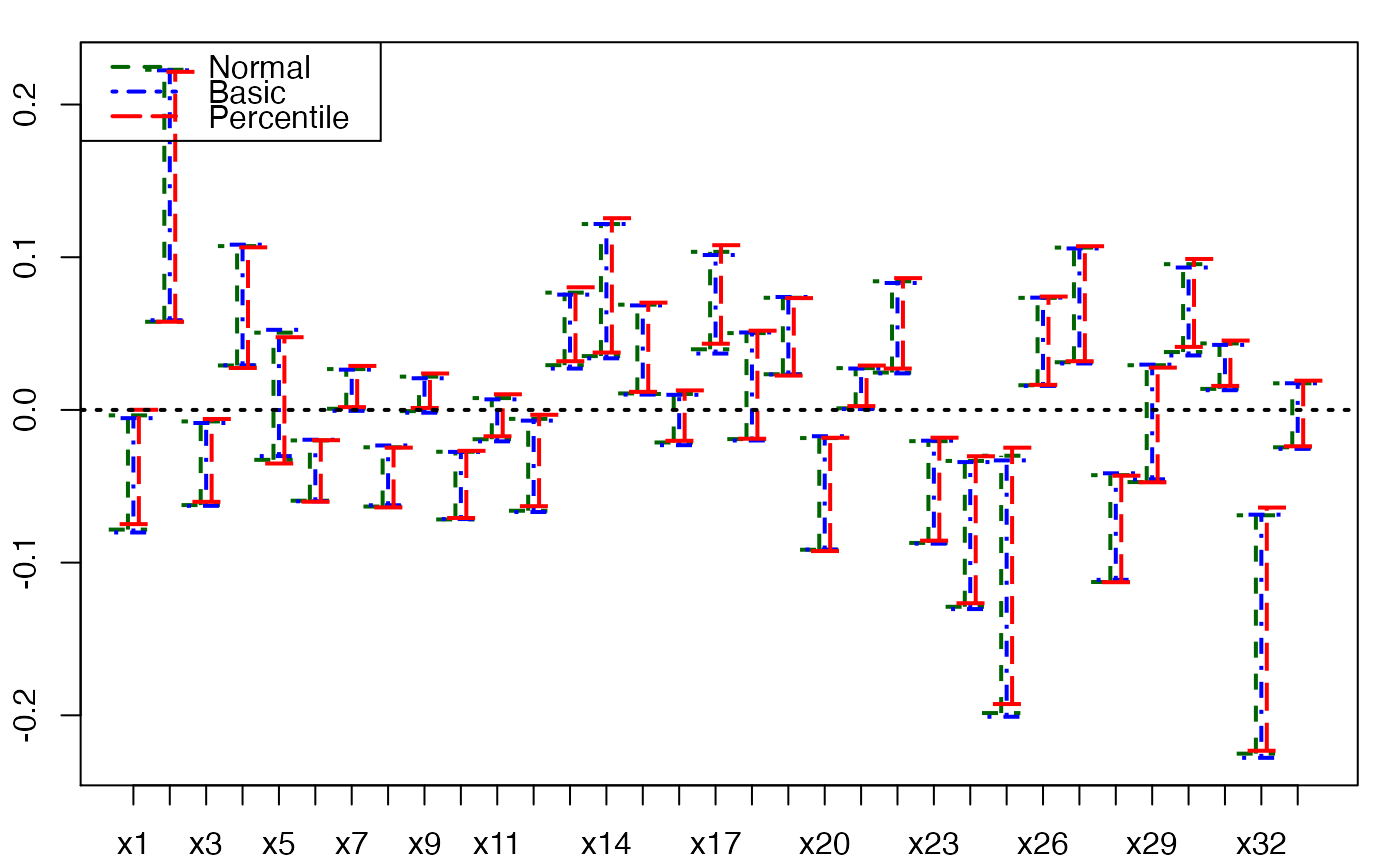
temp.ci <- confints.bootpls(aze_compl.bootYX3,1:34,typeBCa=FALSE)
plots.confints.bootpls(temp.ci,indices=1:33,prednames=FALSE)



# Bastien CSDA 2005 (Y,T) Bootstrap
# much faster
aze_compl.bootYT3 <- bootplsglm(modplsglm, R=1000, verbose=FALSE)
temp.ci <- confints.bootpls(aze_compl.bootYT3)

plots.confints.bootpls(temp.ci)

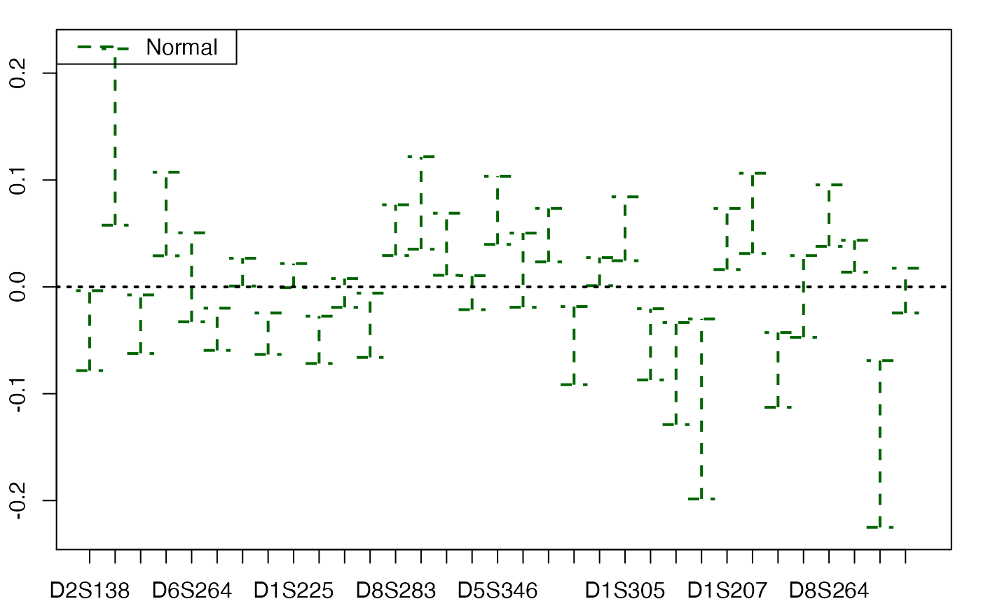
plots.confints.bootpls(temp.ci,typeIC="Normal")

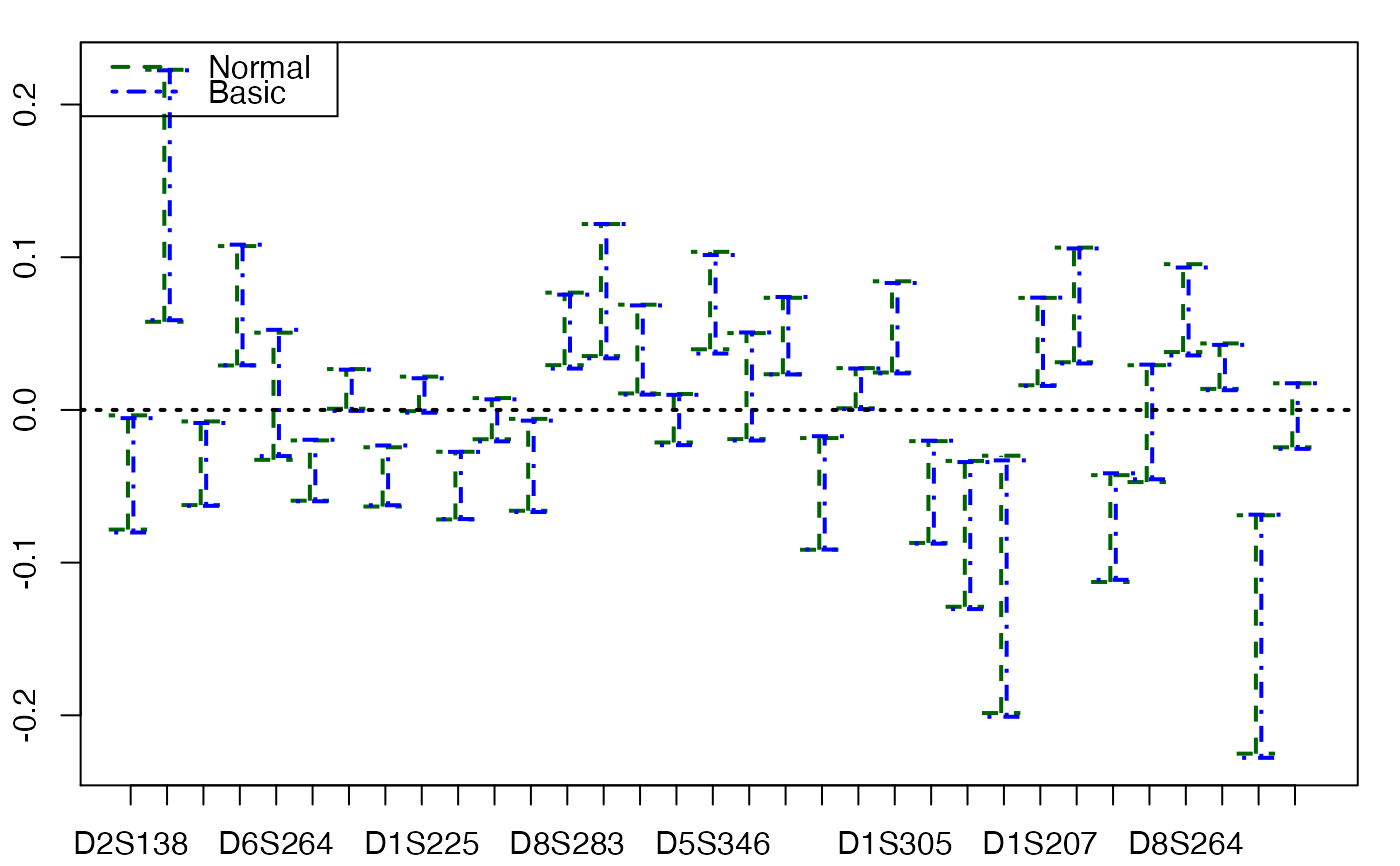
plots.confints.bootpls(temp.ci,typeIC=c("Normal","Basic"))

plots.confints.bootpls(temp.ci,typeIC="BCa",legendpos="bottomleft")

plots.confints.bootpls(temp.ci,prednames=FALSE)

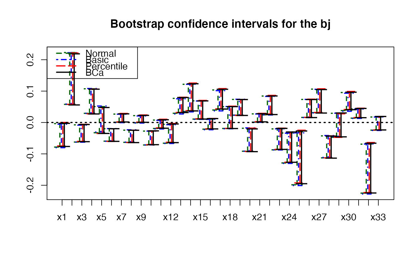
plots.confints.bootpls(temp.ci,prednames=FALSE,articlestyle=FALSE,
main="Bootstrap confidence intervals for the bj")

plots.confints.bootpls(temp.ci,indices=1:33,prednames=FALSE)

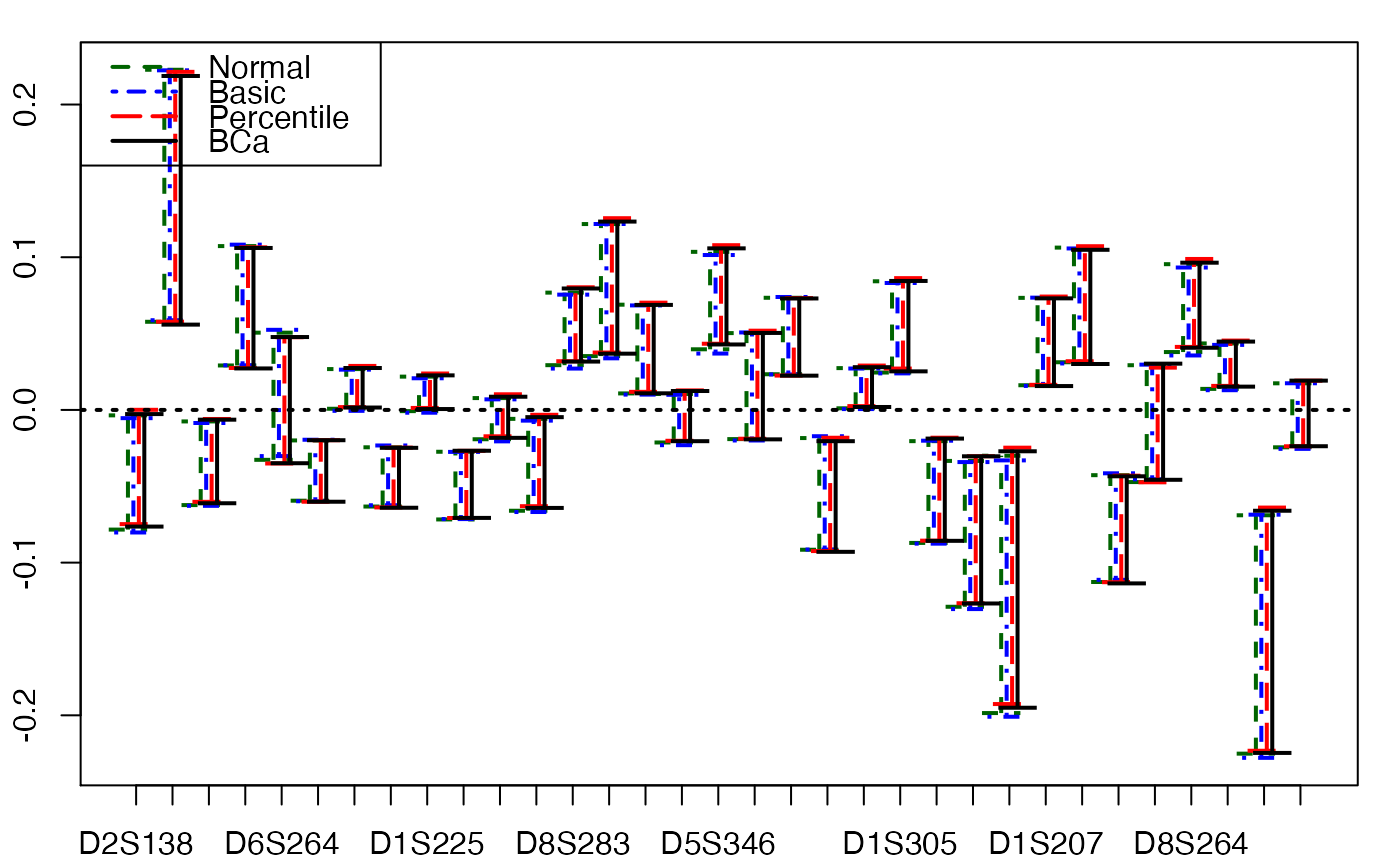
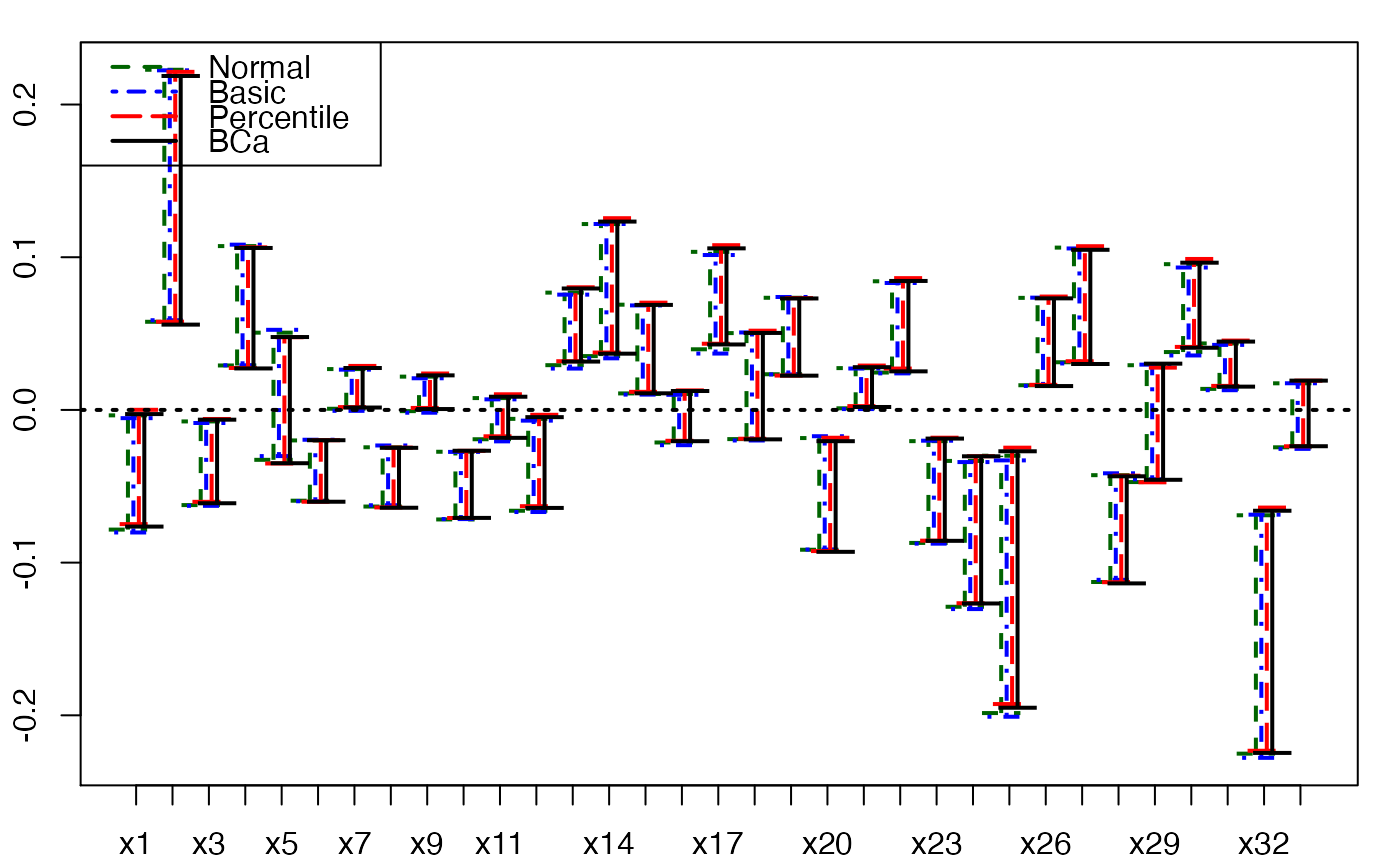
plots.confints.bootpls(temp.ci,c(2,4,6),"bottomleft")

plots.confints.bootpls(temp.ci,c(2,4,6),articlestyle=FALSE,
main="Bootstrap confidence intervals for some of the bj")

plots.confints.bootpls(temp.ci,prednames=FALSE,ltyIC=c(2,1),colIC=c(1,2))

 
temp.ci <- confints.bootpls(aze_compl.bootYT3,1:33,typeBCa=FALSE)
plots.confints.bootpls(temp.ci,prednames=FALSE)

# }

Usage

Arguments

Value

See also

Author

Examples