Comparing SelectBoost-GAMLSS Variants

This vignette compares: plain sb_gamlss, the SelectBoost-integrated SelectBoost_gamlss, grid-based sb_gamlss_c0_grid + autoboost_gamlss, and the lightweight fastboost_gamlss.

What you’ll learn

How the base sb_gamlss() call differs from SelectBoost_gamlss() (automatic grouping).
How to sweep c0 values with sb_gamlss_c0_grid() and let autoboost_gamlss() pick a favourite.
How to generate rapid previews with fastboost_gamlss() before launching a large bootstrap campaign.

library(gamlss)
#> Loading required package: splines
#> Loading required package: gamlss.data
#> 
#> Attaching package: 'gamlss.data'
#> The following object is masked from 'package:datasets':
#> 
#>     sleep
#> Loading required package: gamlss.dist
#> Loading required package: nlme
#> Loading required package: parallel
#>  **********   GAMLSS Version 5.5-0  **********
#> For more on GAMLSS look at https://www.gamlss.com/
#> Type gamlssNews() to see new features/changes/bug fixes.
library(SelectBoost.gamlss)

set.seed(1)
n <- 500
x1 <- rnorm(n); x2 <- rnorm(n); x3 <- rnorm(n); x4 <- rnorm(n)
mu <- 0.5 + 1.2*x1 - 0.8*x3
y  <- gamlss.dist::rNO(n, mu = mu, sigma = 1)
dat <- data.frame(y, x1, x2, x3, x4)

# Baseline
b0 <- sb_gamlss(
  y ~ 1, data = dat, family = gamlss.dist::NO(),
  mu_scope = ~ x1 + x2 + x3 + x4, sigma_scope = ~ x1 + x2,
  B = 50, pi_thr = 0.6, pre_standardize = TRUE, trace = FALSE
)
plot_sb_gamlss(b0)


# SelectBoost integration (single c0)
sb <- SelectBoost_gamlss(
  y ~ 1, data = dat, family = gamlss.dist::NO(),
  mu_scope = ~ x1 + x2 + x3 + x4, sigma_scope = ~ x1 + x2,
  B = 50, pi_thr = 0.6, c0 = 0.5, pre_standardize = TRUE, trace = FALSE
)
summary(sb) |> plot()


# c0 grid + autoboost
g <- sb_gamlss_c0_grid(
  y ~ 1, data = dat, family = gamlss.dist::NO(),
  mu_scope = ~ x1 + x2 + x3 + x4, sigma_scope = ~ x1 + x2,
  c0_grid = seq(0.2, 0.8, by = 0.2), B = 40, pi_thr = 0.6, pre_standardize = TRUE, trace = FALSE
)
#>   |                                                                              |                                                                      |   0%  |                                                                              |==================                                                    |  25%  |                                                                              |===================================                                   |  50%  |                                                                              |====================================================                  |  75%  |                                                                              |======================================================================| 100%
plot(g)

confidence_table(g) |> head()
#>   parameter term conf_index cover
#> 1        mu   x1        0.4     1
#> 5        mu   x3        0.4     1
#> 2     sigma   x1        0.0     0
#> 3        mu   x2        0.0     0
#> 4     sigma   x2        0.0     0
#> 6        mu   x4        0.0     0

ab <- autoboost_gamlss(
  y ~ 1, data = dat, family = gamlss.dist::NO(),
  mu_scope = ~ x1 + x2 + x3 + x4, sigma_scope = ~ x1 + x2,
  c0_grid = seq(0.2, 0.8, by = 0.2), B = 40, pi_thr = 0.6, pre_standardize = TRUE, trace = FALSE
)
#>   |                                                                              |                                                                      |   0%  |                                                                              |==================                                                    |  25%  |                                                                              |===================================                                   |  50%
#> Warning in RS(): Algorithm RS has not yet converged
#>   |                                                                              |====================================================                  |  75%  |                                                                              |======================================================================| 100%
attr(ab, "chosen_c0")
#> [1] 0.2
plot_sb_gamlss(ab)


# fastboost (lightweight)
fb <- fastboost_gamlss(
  y ~ 1, data = dat, family = gamlss.dist::NO(),
  mu_scope = ~ x1 + x2 + x3 + x4, sigma_scope = ~ x1 + x2,
  B = 30, sample_fraction = 0.6, pi_thr = 0.6, pre_standardize = TRUE, trace = FALSE
)
plot_sb_gamlss(fb)

Confidence Functionals (AUSC, Coverage, Quantiles, Weighted, Conservative)

We summarize the stability curves $p_j(c0)$ into single-number scores:

AUSC: normalized area under $p_j(c0)$ across the c0_grid.
Thresholded AUSC ( $(p - \pi^\star)_+$ area): only counts confidence above the stability threshold.
Coverage: fraction of c0 where $p \ge \pi^\star$ .
Quantiles (median/80th/90th): robust distributional summaries of stability.
Weighted AUSC: apply a weight function $w(c0)$ to emphasize parts of the grid.
Conservative AUSC: use Wilson lower bounds for $p$ before computing AUSC.

# Using the grid g created above
cf <- confidence_functionals(
  g, pi_thr = 0.6,
  q = c(0.5, 0.8, 0.9),
  weight_fun = function(c0) (1 - c0)^2,  # emphasize smaller c0
  conservative = TRUE, B = 40,           # use lower bounds
  method = "trapezoid"
)
head(cf)
#>          area  area_pos      w_area cover        sup        inf         q50
#> 1 0.912375461 0.3123755 0.912375461     1 0.91237546 0.91237546 0.912375461
#> 3 0.912375461 0.3123755 0.912375461     1 0.91237546 0.91237546 0.912375461
#> 6 0.048498421 0.0000000 0.063195402     0 0.07061092 0.00000000 0.055094902
#> 5 0.037500329 0.0000000 0.037371182     0 0.05459420 0.02583556 0.039578888
#> 2 0.006910189 0.0000000 0.002892637     0 0.01382038 0.00000000 0.006910189
#> 4 0.000000000 0.0000000 0.000000000     0 0.00000000 0.00000000 0.000000000
#>          q80        q90 parameter term  rank_score
#> 1 0.91237546 0.91237546        mu   x1 0.638662823
#> 3 0.91237546 0.91237546        mu   x3 0.638662823
#> 6 0.07061092 0.07061092     sigma   x2 0.014122183
#> 5 0.04558501 0.05008960     sigma   x1 0.010017921
#> 2 0.01382038 0.01382038        mu   x2 0.002764075
#> 4 0.00000000 0.00000000        mu   x4 0.000000000
plot(cf, top = 12, label_top = 8)


# Inspect stability curves of top terms
top_terms <- head(cf[order(cf$rank_score, decreasing = TRUE), c("term","parameter")], 4)
plot_stability_curves(g, terms = unique(top_terms$term), parameter = unique(top_terms$parameter)[1])

Grouped penalties for factors & splines

library(gamlss)
library(SelectBoost.gamlss)

set.seed(42)
n <- 500
f  <- factor(sample(letters[1:3], n, TRUE))
x1 <- rnorm(n); x2 <- rnorm(n)
y  <- gamlss.dist::rNO(n, mu = 0.3 + 1.2*x1 - 0.7*x2 + 0.5*(f=="c"), sigma = exp(0.1 + 0.2*(f=="b")))

dat <- data.frame(y, f, x1, x2)

# Stepwise baseline
fit_step <- sb_gamlss(
  y ~ 1, data = dat, family = gamlss.dist::NO(),
  mu_scope = ~ f + x1 + pb(x2) + x1:f,
  sigma_scope = ~ f + x1 + pb(x2),
  B = 40, pi_thr = 0.6, pre_standardize = TRUE, trace = FALSE
)

# Group lasso for μ and sparse group lasso for σ
fit_grp <- sb_gamlss(
  y ~ 1, data = dat, family = gamlss.dist::NO(),
  mu_scope = ~ f + x1 + pb(x2) + x1:f,
  sigma_scope = ~ f + x1 + pb(x2),
  engine = "grpreg", engine_sigma = "sgl",
  B = 40, pi_thr = 0.6, pre_standardize = TRUE, trace = FALSE
)

plot_sb_gamlss(fit_step)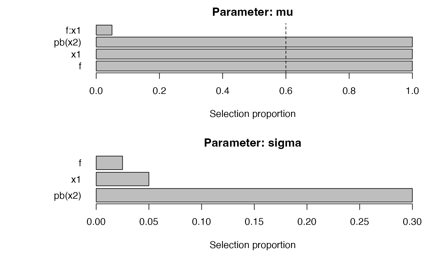

plot_sb_gamlss(fit_grp)

selection_table(fit_step) |> head()
#>   parameter   term count  prop
#> 1        mu      f    40 1.000
#> 2        mu     x1    40 1.000
#> 3        mu pb(x2)    40 1.000
#> 4        mu   f:x1     2 0.050
#> 5     sigma      f     1 0.025
#> 6     sigma     x1     2 0.050
selection_table(fit_grp)  |> head()
#>   parameter   term count prop
#> 1        mu      f     0    0
#> 2        mu     x1     0    0
#> 3        mu pb(x2)     0    0
#> 4        mu   f:x1     0    0
#> 5     sigma      f    40    1
#> 6     sigma     x1    40    1

Tuning & Group Knockoffs

# Tuning engines / penalties
cfgs <- list(
  list(engine="stepGAIC"),
  list(engine="glmnet", glmnet_alpha=1),
  list(engine="grpreg", grpreg_penalty="grLasso", engine_sigma="sgl", sgl_alpha=0.9)
)
base <- list(
  formula = y ~ 1, data = dat, family = gamlss.dist::NO(),
  mu_scope = ~ f + x1 + pb(x2) + x1:f, sigma_scope = ~ f + x1 + pb(x2),
  pi_thr = 0.6, pre_standardize = TRUE, sample_fraction = 0.7, parallel = "auto", trace = FALSE
)
tuned <- tune_sb_gamlss(cfgs, base_args = base, B_small = 30)
#>   |                                                                              |                                                                      |   0%  |                                                                              |=======================                                               |  33%  |                                                                              |===============================================                       |  67%  |                                                                              |======================================================================| 100%
tuned$best_config
#> $engine
#> [1] "stepGAIC"

# Approximate group knockoffs for mu
sel_mu <- NULL
if (requireNamespace("knockoff", quietly = TRUE)) {
  sel_mu <- tryCatch(
    knockoff_filter_mu(dat, response = "y", mu_scope = ~ f + x1 + pb(x2), fdr = 0.1),
    error = function(e) {
      cat("Knockoff filter failed:", conditionMessage(e), "— skipping example.\n")
      NULL
    }
  )
} else {
  cat("Package 'knockoff' not installed; skipping knockoff example.\n")
}
#> Knockoff filter failed: non-numeric argument to binary operator — skipping example.
if (!is.null(sel_mu)) sel_mu

Frédéric Bertrand

2025-10-27

What you’ll learn

Confidence Functionals (AUSC, Coverage, Quantiles, Weighted, Conservative)

Grouped penalties for factors & splines

Tuning & Group Knockoffs