Confidence Functionals for SelectBoost-GAMLSS

Frédéric Bertrand

Cedric, Cnam, Paris
frederic.bertrand@lecnam.net

2025-10-27

We consider stability curves $p_j(c0)$ for each term $j$ across a grid of SelectBoost thresholds c0. The following functionals condense these curves into scalar confidences:

What you’ll learn

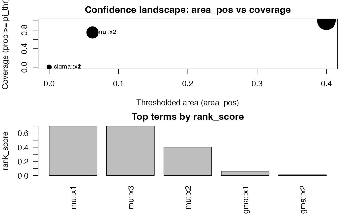
• How to compute confidence_functionals() from a sb_gamlss_c0_grid() result.
• How to plot ranking summaries (plot()) and raw stability trajectories (plot_stability_curves()).
• How to customise weights, quantiles, and conservative adjustments for different decision rules.

1. AUSC (Area Under the Stability Curve): normalized trapezoidal area over the grid.
2. Thresholded AUSC: integrate the positive excess $(p - \pi^\star)_+$.
3. Coverage: fraction of grid points with $p \ge \pi^\star$.
4. Quantiles: median and high quantiles (e.g., 80th/90th) of $p$ across c0.
5. Weighted AUSC: integrate $w(c0)\,p(c0)$ normalized by $\int w(c0)\,dc0$.
6. Conservative AUSC: replace $p$ by a Wilson lower bound before integrating.

library(gamlss)
#> Loading required package: splines
#> Loading required package: gamlss.data
#> 
#> Attaching package: 'gamlss.data'
#> The following object is masked from 'package:datasets':
#> 
#>     sleep
#> Loading required package: gamlss.dist
#> Loading required package: nlme
#> Loading required package: parallel
#>  **********   GAMLSS Version 5.5-0  **********
#> For more on GAMLSS look at https://www.gamlss.com/
#> Type gamlssNews() to see new features/changes/bug fixes.
library(SelectBoost.gamlss)

set.seed(1)
n <- 400
x1 <- rnorm(n); x2 <- rnorm(n); x3 <- rnorm(n)
y  <- gamlss.dist::rNO(n, mu = 1 + 1.3*x1 - 1.0*x3, sigma = 1)
dat <- data.frame(y, x1, x2, x3)

g <- sb_gamlss_c0_grid(
  y ~ 1, data = dat, family = gamlss.dist::NO(),
  mu_scope = ~ x1 + x2 + x3, sigma_scope = ~ x1 + x2,
  c0_grid = seq(0.2, 0.8, by = 0.2), B = 40, pi_thr = 0.6, pre_standardize = TRUE, trace = FALSE
)
#>   |                                                                              |                                                                      |   0%  |                                                                              |==================                                                    |  25%  |                                                                              |===================================                                   |  50%
#> Warning in RS(): Algorithm RS has not yet converged
#>   |                                                                              |====================================================                  |  75%  |                                                                              |======================================================================| 100%

cf <- confidence_functionals(
  g, pi_thr = 0.6, q = c(0.5, 0.8, 0.9),
  weight_fun = NULL, conservative = FALSE, method = "trapezoid"
)

plot(cf, top = 10, label_top = 6)

plot_stability_curves(g, terms = c("x1","x3"), parameter = "mu")