Real Data Examples with Different Distributions
Frédéric Bertrand
Cedric, Cnam, Parisfrederic.bertrand@lecnam.net
2025-12-03
Source:vignettes/real-data-examples.Rmd
real-data-examples.RmdThis vignette demonstrates SelectBoost.gamlss on real datasets using different distributions. We include a growth example (Dutch boys) and further count/continuous/binary cases.
What you’ll learn
- How to configure scopes and engines for Box–Cox t growth models, insurance claims, and quine attendance.
- How to use
selection_table()andeffect_plot()to interpret the resulting fits. - How to adjust bootstrap settings (
B,pi_thr,parallel) for heavier real-world analyses.
You may want to install optional engines for best results:
install.packages(c("glmnet","grpreg","SGL","future.apply"))
library(SelectBoost.gamlss)
library(gamlss)
#> Loading required package: splines
#> Loading required package: gamlss.data
#>
#> Attaching package: 'gamlss.data'
#> The following object is masked from 'package:datasets':
#>
#>     sleep
#> Loading required package: gamlss.dist
#> Loading required package: nlme
#> Loading required package: parallel
#>  **********   GAMLSS Version 5.5-0  **********
#> For more on GAMLSS look at https://www.gamlss.com/
#> Type gamlssNews() to see new features/changes/bug fixes.
library(MASS)           # Insurance, quine
set.seed(1)
1. Growth data (BCT) — Dutch boys
We model height vs age with BCT (Box–Cox t). Grouped penalties select among smoothers and interactions with pubertal stage.
Increase B to 50 for real use.
set.seed(123)
# Load and CLEAN the Dutch boys growth data
utils::data("boys7482", package = "SelectBoost.gamlss")
# Keep only rows complete
boys <- boys7482[stats::complete.cases(boys7482),]
boys$gen <- as.factor(boys$gen)
# (Optional) keep levels actually present
boys <- droplevels(boys)
# Fit SelectBoost.gamlss on CLEANED data (no parallel for vignette stability)
fit_growth <- sb_gamlss(
hgt ~ 1, data = boys, family = gamlss.dist::BCT(),
mu_scope = ~ pb(age) + pb(age):gen,
sigma_scope = ~ pb(age),
nu_scope = ~ pb(age),
engine = "grpreg", engine_sigma = "grpreg", engine_nu = "grpreg",
grpreg_penalty = "grLasso",
B = 1, pi_thr = 0.6, pre_standardize = TRUE,
parallel = "none", trace = FALSE
)
# Peek at selection (first rows)
print(utils::head(selection_table(fit_growth), 12))
#> parameter term count prop
#> 1 mu pb(age) 0 0
#> 2 mu pb(age):gen 0 0
#> 3 sigma pb(age) 0 0
#> 4 nu pb(age) 0 0
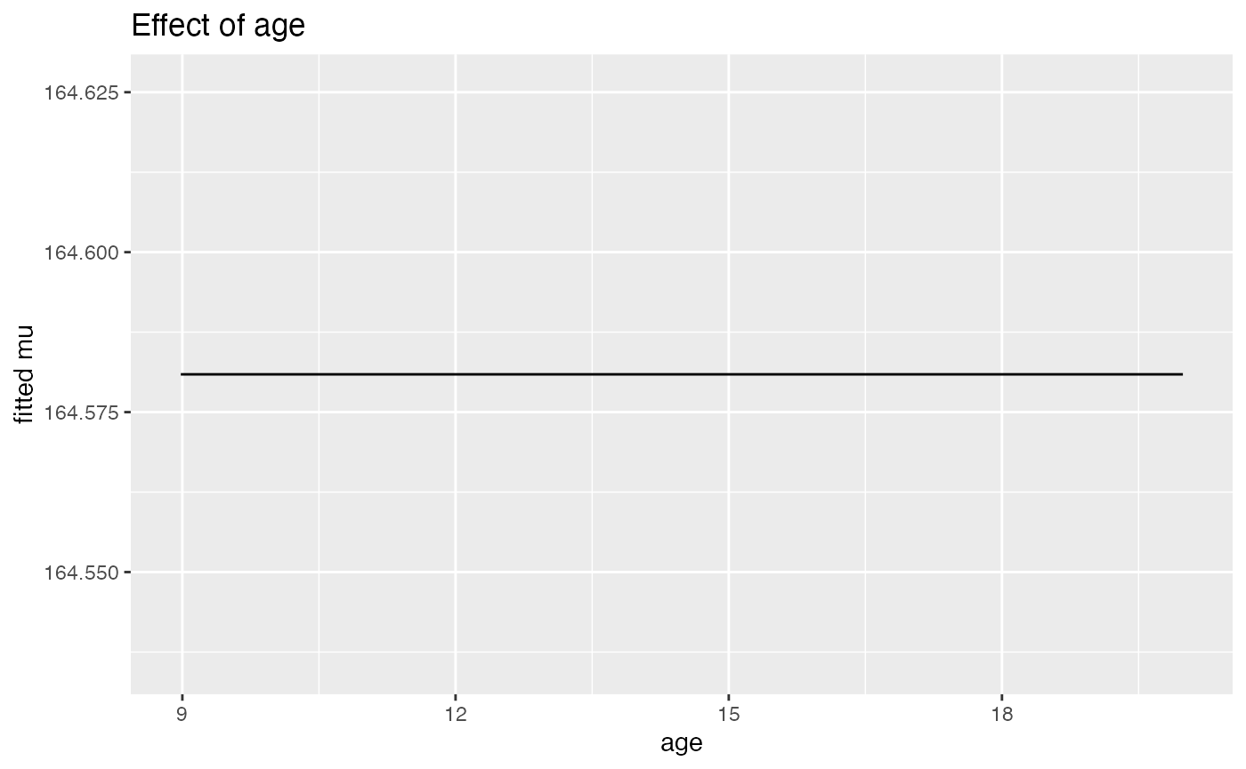
# Effect plot for age on mu
if (requireNamespace("ggplot2", quietly = TRUE)) {
print(effect_plot(fit_growth, "age", boys, what = "mu"))
}
Increase B to 50 for real use.
set.seed(123)
# Stability curves over a small c0 grid (still on CLEANED data)
  g <- sb_gamlss_c0_grid(
    hgt ~ 1, data = boys, family = gamlss.dist::BCT(),
    mu_scope = ~ pb(age) + pb(age):gen,
    sigma_scope = ~ pb(age),
    nu_scope = ~ pb(age),
    c0_grid = seq(0.2, 0.8, by = 0.1),
    B = 1, pi_thr = 0.6, pre_standardize = TRUE,
    parallel = "none", trace = FALSE
  )
  plot_stability_curves(g, terms = c("pb(age)", "pb(age):gen"), parameter = "mu")
Interpretation. Expect pb(age) to be
stably selected for μ and σ; interactions like pb(age):gen
often appear around puberty.
2. Count data (PO) — Insurance claims
Fit Poisson with log-offset for exposure.
data(Insurance, package = "MASS")
ins <- transform(Insurance, logH = log(Holders))
fit_po <- sb_gamlss(
Claims ~ offset(logH), data = ins, family = gamlss.dist::PO(),
mu_scope = ~ Age + District + Group,
engine = "glmnet", glmnet_alpha = 1, # lasso
B = 100, pi_thr = 0.6, pre_standardize = FALSE,
parallel = "auto", trace = FALSE
)
selection_table(fit_po)
#> parameter term count prop
#> 1 mu Age 100 1
#> 2 mu District 100 1
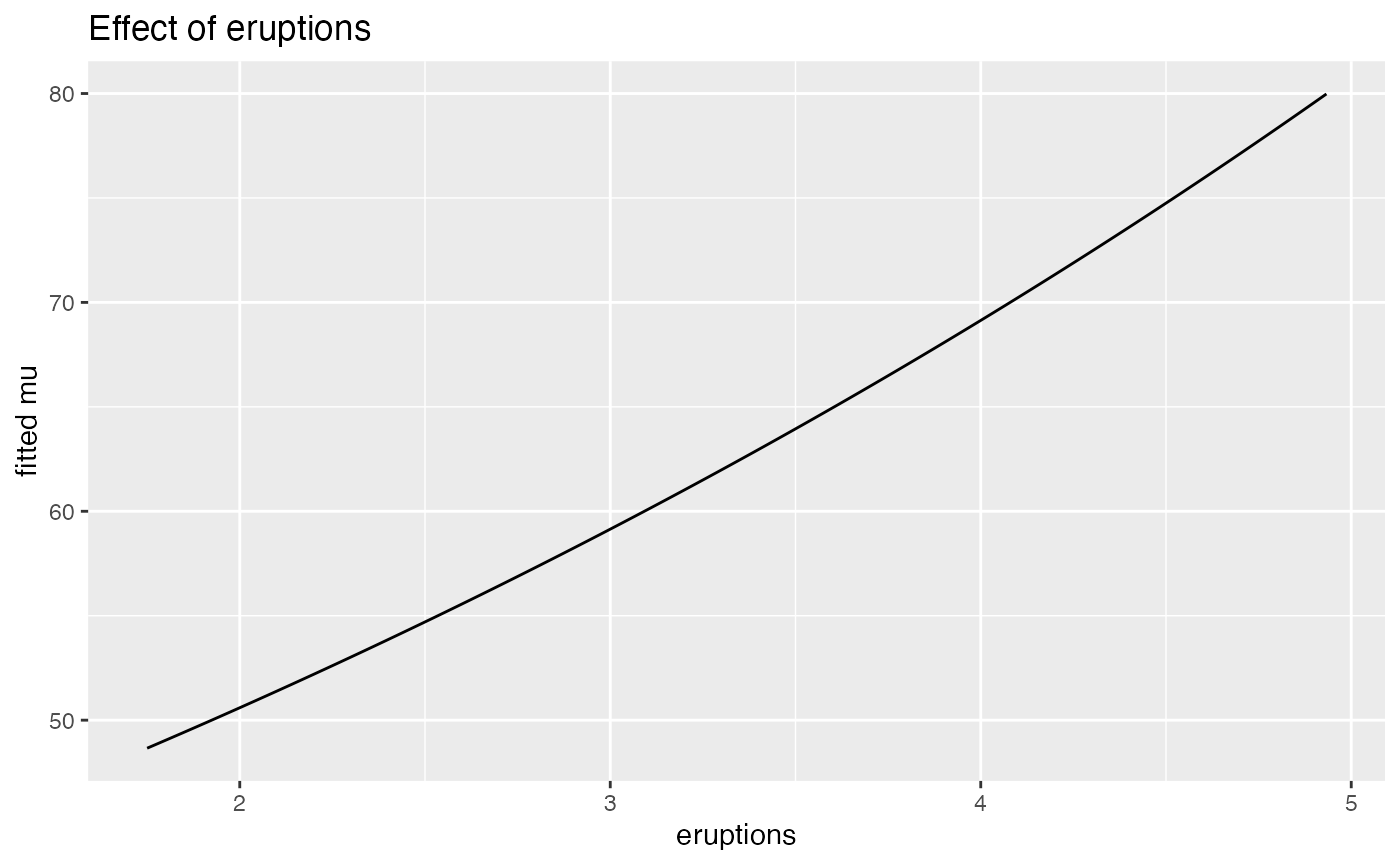
#> 3 mu Group 100 13. Positive continuous (GA) — Old Faithful
Use Gamma for positive waiting times vs eruption length.
data(faithful)
faith <- transform(faithful, eru2 = eruptions^2)

fit_ga <- sb_gamlss(
  waiting ~ 1, data = faith, family = gamlss.dist::GA(),
  mu_scope    = ~ pb(eruptions) + eru2,
  sigma_scope = ~ pb(eruptions),
  engine = "glmnet", glmnet_alpha = 0.5,   # elastic-net
  B = 60, pi_thr = 0.6, pre_standardize = TRUE,
  parallel = "auto", trace = FALSE
)

selection_table(fit_ga)
#>   parameter          term count prop
#> 1        mu pb(eruptions)    60    1
#> 2        mu          eru2    60    1
#> 3     sigma pb(eruptions)    60    1
# Effect plot for eruptions on mu
if (requireNamespace('ggplot2', quietly = TRUE)) {
  print(effect_plot(fit_ga, 'eruptions', faith, what = 'mu'))
}
4. Binary (BI) — mtcars transmission
Treat am (0/1) as Bernoulli.
mt <- transform(mtcars,
  am = as.integer(am),
  cyl = factor(cyl), gear = factor(gear), carb = factor(carb), vs = factor(vs))

fit_bin <- sb_gamlss(
  am ~ 1, data = mt, family = gamlss.dist::BI(),
  mu_scope = ~ wt + hp + qsec + cyl + gear + carb + vs,
  engine = "grpreg", grpreg_penalty = "grLasso",
  B = 80, pi_thr = 0.6, pre_standardize = TRUE,
  parallel = "auto", trace = FALSE
)

selection_table(fit_bin)
#>   parameter term count prop
#> 1        mu   wt     0    0
#> 2        mu   hp     0    0
#> 3        mu qsec     0    0
#> 4        mu  cyl     0    0
#> 5        mu gear     0    0
#> 6        mu carb     0    0
#> 7        mu   vs     0    0
5. Overdispersed counts (NBII) — quine absences
Negative Binomial II handles extra-Poisson variation.
data(quine, package = "MASS")
fit_nb2 <- sb_gamlss(
  Days ~ 1, data = quine, family = gamlss.dist::NBII(),
  mu_scope = ~ Eth + Sex + Lrn + Age,
  engine = "grpreg", grpreg_penalty = "grLasso",
  B = 80, pi_thr = 0.6, pre_standardize = FALSE,
  parallel = "auto", trace = FALSE
)

selection_table(fit_nb2)
#>   parameter term count prop
#> 1        mu  Eth     0    0
#> 2        mu  Sex     0    0
#> 3        mu  Lrn     0    0
#> 4        mu  Age     0    0
Tips
- If you have many factor levels or smoothers, prefer
engine="grpreg"/"sgl"(group-aware). - For very wide numeric designs, try
engine="glmnet"withglmnet_alphain . - Use
pre_standardize=TRUE(fast C++ scaler) when predictors are numeric and on different scales. - For speed, enable parallel workers:
future::plan(multisession, workers = 4); parallel="auto".