Fast big-memory workflows with bigPLScox
Frédéric Bertrand
Cedric, Cnam, Parisfrederic.bertrand@lecnam.net
2025-11-16
Source:vignettes/bigPLScox.Rmd
bigPLScox.RmdIntroduction
Large survival datasets often outgrow the capabilities of purely in-memory algorithms. bigPLScox therefore offers three flavours of Partial Least Squares (PLS) components for Cox models:
-
big_pls_cox()– the original R/C++ hybrid that expects dense matrices; -
big_pls_cox_fast()– the new Armadillo backend with variance-one components and support for both dense matrices andbigmemory::big.matrixobjects; and -
big_pls_cox_gd()– a stochastic gradient descent (SGD) solver for streaming or disk-backed data. allowing datasets too large to fit in RAM.
This vignette demonstrates how to build file-backed matrices, run the
fast backends, and reconcile their outputs. It complements the
introductory vignette
vignette("getting-started", package = "bigPLScox") and
focuses on workflow patterns specific to large datasets.
Simulating a large survival dataset
We generate a synthetic dataset with correlated predictors and a known linear predictor. The same object is used to illustrate the dense and big-memory interfaces.
library(bigPLScox)
set.seed(2024)

n_obs  <- 5000
n_pred <- 100
k_true <- 3

Sigma <- diag(n_pred)
for (b in 0:2) {
  idx <- (b * 10 + 1):(b * 10 + 10)
  Sigma[idx, idx] <- 0.7
  diag(Sigma[idx, idx]) <- 1
}

L <- chol(Sigma)
Z <- matrix(rnorm(n_obs * n_pred), nrow = n_obs)
X_dense <- Z %*% L

w1 <- numeric(n_pred); w1[1:4]   <- c( 1.0,  0.8,  0.6, -0.5)
w2 <- numeric(n_pred); w2[5:8]   <- c(-0.7,  0.9, -0.4,  0.5)
w3 <- numeric(n_pred); w3[9:12]  <- c( 0.6, -0.5,  0.7,  0.8)
w1 <- w1 / sqrt(sum(w1^2))
w2 <- w2 / sqrt(sum(w2^2))
w3 <- w3 / sqrt(sum(w3^2))

t1 <- as.numeric(scale(drop(X_dense %*% w1), center = TRUE, scale = TRUE))
t2 <- as.numeric(scale(drop(X_dense %*% w2), center = TRUE, scale = TRUE))
t3 <- as.numeric(scale(drop(X_dense %*% w3), center = TRUE, scale = TRUE))

beta_true <- c(1.0, 0.6, 0.3)
eta       <- beta_true[1]*t1 + beta_true[2]*t2 + beta_true[3]*t3

lambda0 <- 0.05
u <- runif(n_obs)
time_event <- -log(u) / (lambda0 * exp(eta))

target_event <- 0.65

f <- function(lc) {
  mean(time_event <= rexp(n_obs, rate = lc)) - target_event
}
lambda_c <- uniroot(f, c(1e-4, 1), tol = 1e-4)$root
time_cens <- rexp(n_obs, rate = lambda_c)

time   <- pmin(time_event, time_cens)
status <- as.integer(time_event <= time_cens)
if (requireNamespace("bigmemory", quietly = TRUE)) {
  library(bigmemory)
  big_dir <- tempfile("bigPLScox-")
  dir.create(big_dir)
  if(file.exists(paste(big_dir,"X.bin",sep="/"))){unlink(paste(big_dir,"X.bin",sep="/"))}
  if(file.exists(paste(big_dir,"X.desc",sep="/"))){unlink(paste(big_dir,"X.desc",sep="/"))}
  X_big <- bigmemory::as.big.matrix(
    X_dense,
    backingpath = big_dir,
    backingfile = "X.bin",
    descriptorfile = "X.desc"
  )
  X_big[1:6, 1:6]
}
#>            [,1]       [,2]       [,3]       [,4]       [,5]       [,6]
#> [1,]  0.9819694  1.1785102  0.8893563  0.4103456  0.8595229  1.2643346
#> [2,]  0.4687150  0.3552132  0.1072107  0.7865815  0.6736797  0.9825877
#> [3,] -0.1079713 -0.9804778 -1.7053786 -0.3227459 -0.6558693  0.4394022
#> [4,] -0.2128782  0.1114703 -0.8085431 -0.7675984 -0.3685458 -0.7628635
#> [5,]  1.1580985  1.0561296  1.1652026  1.5047814  0.3721924  1.1937471
#> [6,]  1.2923548  1.2431242  1.1954762  1.7104007  1.7505597  0.3548417
Dense-matrix solvers
The legacy solver big_pls_cox() performs the component
extraction in R before fitting the Cox model. The new
big_pls_cox_fast() backend exposes the same arguments but
runs entirely in C++ for a substantial speed-up.
fit_legacy <- big_pls_cox(
  X = X_dense,
  time = time,
  status = status,
  ncomp = k_true
)
fit_fast_dense <- big_pls_cox_fast(
  X = X_dense,
  time = time,
  status = status,
  ncomp = k_true
)

list(
  legacy = head(fit_legacy$scores),
  fast = head(fit_fast_dense$scores)
)
#> $legacy
#>            [,1]         [,2]       [,3]
#> [1,]  0.9629914 -0.167053846  0.7375230
#> [2,]  0.2108181 -0.770048070 -0.7462166
#> [3,] -0.6636008  0.469979735 -0.5996875
#> [4,] -0.4659735  0.004452889 -0.5171283
#> [5,]  1.1370381 -1.060165048  0.4919368
#> [6,]  1.1498123  0.643174881 -2.0723580
#>
#> $fast
#>            [,1]        [,2]        [,3]
#> [1,]  0.9687369  0.08567234  0.55026138
#> [2,]  0.2084113 -0.27560071 -0.81298189
#> [3,] -0.6452360  0.17006440 -0.59713551
#> [4,] -0.3704446 -1.74944701 -0.56995206
#> [5,]  1.1710374 -0.97228981 -0.09285005
#> [6,]  1.1309082  1.29090796 -1.67416198

list(
  legacy = apply(fit_legacy$scores, 2, var),
  fast = apply(fit_fast_dense$scores, 2, var)
)
#> $legacy
#> [1] 1 1 1
#>
#> $fast
#> [1] 1 1 1
The summary() method reports key diagnostics, including
the final Cox coefficients and the number of predictors retained per
component.
summary(fit_fast_dense)
#> $n
#> [1] 5000
#>
#> $p
#> [1] 100
#>
#> $ncomp
#> [1] 3
#>
#> $keepX
#> [1] 0 0 0
#>
#> $center
#>   [1]  2.798955e-03 -9.107153e-03 -2.635946e-03 -4.943362e-03 -7.487132e-03
#>   [6]  1.688500e-03  1.210463e-02 -3.535210e-03  7.937559e-03 -5.111552e-03
#>  [11]  2.432002e-02  2.761799e-02  1.006852e-02  1.894906e-02  5.913826e-03
#>  [16]  1.760013e-02  2.038917e-02  1.990905e-02  8.037810e-03  1.348481e-02
#>  [21] -8.386266e-04 -1.395535e-02  1.267194e-03  4.733988e-03 -3.000423e-03
#>  [26]  4.522036e-03  1.537932e-02  7.581824e-03  1.149183e-02  8.462248e-05
#>  [31]  5.932423e-03 -1.466198e-02 -1.034713e-02 -1.481074e-02 -2.251482e-02
#>  [36]  1.509019e-02  7.071338e-03  1.671894e-03 -5.115363e-04  7.012307e-03
#>  [41]  1.064288e-02  9.916201e-03 -6.026108e-03  5.773966e-03  4.633769e-03
#>  [46]  2.618328e-02 -1.435784e-02 -5.742304e-03 -1.915827e-02  8.912658e-03
#>  [51]  9.885805e-04 -2.480366e-02 -2.473665e-02  1.140294e-02 -1.765096e-03
#>  [56]  1.098523e-02  1.313620e-02  1.197506e-02  1.582672e-02 -1.068739e-02
#>  [61]  2.012116e-02 -2.190880e-03 -1.949041e-02  1.068698e-02  2.140322e-03
#>  [66] -1.930552e-02 -8.015752e-03  4.882372e-03  9.592623e-03  6.027325e-03
#>  [71]  1.753572e-02 -7.224351e-03  3.237467e-02  2.087540e-02 -1.771835e-02
#>  [76]  1.911843e-02  4.837475e-03 -4.556118e-03 -3.789627e-03 -1.290946e-02
#>  [81] -2.352335e-03 -1.463869e-02 -6.529425e-03 -2.007038e-04 -2.049618e-02
#>  [86]  9.593425e-03 -4.618771e-03 -3.091546e-02 -4.459583e-03  1.441065e-02
#>  [91]  1.209319e-02 -1.910077e-02 -2.138175e-03 -8.270438e-03 -6.362283e-04
#>  [96]  1.212042e-02  1.317364e-02  6.920960e-03 -2.154896e-02 -7.828461e-03
#>
#> $scale
#>   [1] 0.9910953 0.9879135 0.9801627 0.9805454 0.9825838 0.9796072 0.9916807
#>   [8] 0.9639126 0.9752288 0.9795114 1.0061235 1.0183937 1.0153322 1.0055659
#>  [15] 0.9999027 0.9982914 1.0180898 0.9965759 0.9989057 0.9980811 0.9831231
#>  [22] 0.9932899 0.9880039 0.9783728 0.9910691 0.9997550 0.9942396 0.9809138
#>  [29] 0.9849191 0.9897065 0.9945993 1.0059848 1.0222768 1.0053630 0.9941951
#>  [36] 1.0161263 0.9891056 0.9935245 1.0022409 1.0132022 1.0015934 1.0014491
#>  [43] 0.9971142 0.9969146 1.0076407 1.0089492 0.9954433 1.0043024 1.0001044
#>  [50] 1.0135577 0.9882588 0.9739312 1.0097109 0.9841654 1.0101256 1.0137299
#>  [57] 1.0081388 0.9964486 0.9813350 0.9899351 0.9940586 1.0100280 0.9865722
#>  [64] 1.0140406 1.0073922 0.9988660 0.9999025 0.9958502 0.9915252 1.0199301
#>  [71] 0.9953438 1.0018892 1.0034691 1.0040947 1.0079260 0.9916430 1.0128318
#>  [78] 1.0173742 1.0159493 0.9991616 1.0117705 1.0176843 1.0043697 0.9917577
#>  [85] 1.0073844 0.9954760 0.9968360 0.9983667 0.9877749 0.9831503 1.0071013
#>  [92] 1.0195985 1.0051072 0.9875478 1.0110776 0.9969945 0.9953462 0.9948409
#>  [99] 0.9953168 0.9914863
#>
#> $cox
#> Call:
#> survival::coxph(formula = survival::Surv(time, status) ~ ., data = scores_df,
#>     ties = "efron", x = FALSE)
#>
#>   n= 5000, number of events= 3250
#>
#>           coef exp(coef) se(coef)      z Pr(>|z|)
#> comp1  1.01373   2.75587  0.02115  47.94   <2e-16 ***
#> comp2 -0.41079   0.66313  0.01792 -22.92   <2e-16 ***
#> comp3  0.20389   1.22617  0.01804  11.30   <2e-16 ***
#> ---
#> Signif. codes:  0 '***' 0.001 '**' 0.01 '*' 0.05 '.' 0.1 ' ' 1
#>
#>       exp(coef) exp(-coef) lower .95 upper .95
#> comp1    2.7559     0.3629    2.6440    2.8725
#> comp2    0.6631     1.5080    0.6402    0.6868
#> comp3    1.2262     0.8155    1.1836    1.2703
#>
#> Concordance= 0.765  (se = 0.004 )
#> Likelihood ratio test= 2757  on 3 df,   p=<2e-16
#> Wald test            = 2669  on 3 df,   p=<2e-16
#> Score (logrank) test = 2680  on 3 df,   p=<2e-16
#>
#>
#> attr(,"class")
#> [1] "summary.big_pls_cox"
Switching to file-backed matrices
When working with a big.matrix, the same function
operates on the shared memory pointer without copying data back to R.
This is ideal for datasets that do not fit entirely in RAM.
if (exists("X_big")) {
  fit_fast_big <- big_pls_cox_fast(
    X = X_big,
    time = time,
    status = status,
    ncomp = k_true
  )
  summary(fit_fast_big)
}
#> $n
#> [1] 5000
#>
#> $p
#> [1] 100
#>
#> $ncomp
#> [1] 3
#>
#> $keepX
#> [1] 0 0 0
#>
#> $center
#>   [1]  2.798955e-03 -9.107153e-03 -2.635946e-03 -4.943362e-03 -7.487132e-03
#>   [6]  1.688500e-03  1.210463e-02 -3.535210e-03  7.937559e-03 -5.111552e-03
#>  [11]  2.432002e-02  2.761799e-02  1.006852e-02  1.894906e-02  5.913826e-03
#>  [16]  1.760013e-02  2.038917e-02  1.990905e-02  8.037810e-03  1.348481e-02
#>  [21] -8.386266e-04 -1.395535e-02  1.267194e-03  4.733988e-03 -3.000423e-03
#>  [26]  4.522036e-03  1.537932e-02  7.581824e-03  1.149183e-02  8.462248e-05
#>  [31]  5.932423e-03 -1.466198e-02 -1.034713e-02 -1.481074e-02 -2.251482e-02
#>  [36]  1.509019e-02  7.071338e-03  1.671894e-03 -5.115363e-04  7.012307e-03
#>  [41]  1.064288e-02  9.916201e-03 -6.026108e-03  5.773966e-03  4.633769e-03
#>  [46]  2.618328e-02 -1.435784e-02 -5.742304e-03 -1.915827e-02  8.912658e-03
#>  [51]  9.885805e-04 -2.480366e-02 -2.473665e-02  1.140294e-02 -1.765096e-03
#>  [56]  1.098523e-02  1.313620e-02  1.197506e-02  1.582672e-02 -1.068739e-02
#>  [61]  2.012116e-02 -2.190880e-03 -1.949041e-02  1.068698e-02  2.140322e-03
#>  [66] -1.930552e-02 -8.015752e-03  4.882372e-03  9.592623e-03  6.027325e-03
#>  [71]  1.753572e-02 -7.224351e-03  3.237467e-02  2.087540e-02 -1.771835e-02
#>  [76]  1.911843e-02  4.837475e-03 -4.556118e-03 -3.789627e-03 -1.290946e-02
#>  [81] -2.352335e-03 -1.463869e-02 -6.529425e-03 -2.007038e-04 -2.049618e-02
#>  [86]  9.593425e-03 -4.618771e-03 -3.091546e-02 -4.459583e-03  1.441065e-02
#>  [91]  1.209319e-02 -1.910077e-02 -2.138175e-03 -8.270438e-03 -6.362283e-04
#>  [96]  1.212042e-02  1.317364e-02  6.920960e-03 -2.154896e-02 -7.828461e-03
#>
#> $scale
#>   [1] 0.9910953 0.9879135 0.9801627 0.9805454 0.9825838 0.9796072 0.9916807
#>   [8] 0.9639126 0.9752288 0.9795114 1.0061235 1.0183937 1.0153322 1.0055659
#>  [15] 0.9999027 0.9982914 1.0180898 0.9965759 0.9989057 0.9980811 0.9831231
#>  [22] 0.9932899 0.9880039 0.9783728 0.9910691 0.9997550 0.9942396 0.9809138
#>  [29] 0.9849191 0.9897065 0.9945993 1.0059848 1.0222768 1.0053630 0.9941951
#>  [36] 1.0161263 0.9891056 0.9935245 1.0022409 1.0132022 1.0015934 1.0014491
#>  [43] 0.9971142 0.9969146 1.0076407 1.0089492 0.9954433 1.0043024 1.0001044
#>  [50] 1.0135577 0.9882588 0.9739312 1.0097109 0.9841654 1.0101256 1.0137299
#>  [57] 1.0081388 0.9964486 0.9813350 0.9899351 0.9940586 1.0100280 0.9865722
#>  [64] 1.0140406 1.0073922 0.9988660 0.9999025 0.9958502 0.9915252 1.0199301
#>  [71] 0.9953438 1.0018892 1.0034691 1.0040947 1.0079260 0.9916430 1.0128318
#>  [78] 1.0173742 1.0159493 0.9991616 1.0117705 1.0176843 1.0043697 0.9917577
#>  [85] 1.0073844 0.9954760 0.9968360 0.9983667 0.9877749 0.9831503 1.0071013
#>  [92] 1.0195985 1.0051072 0.9875478 1.0110776 0.9969945 0.9953462 0.9948409
#>  [99] 0.9953168 0.9914863
#>
#> $cox
#> Call:
#> survival::coxph(formula = survival::Surv(time, status) ~ ., data = scores_df,
#>     ties = "efron", x = FALSE)
#>
#>   n= 5000, number of events= 3250
#>
#>           coef exp(coef) se(coef)      z Pr(>|z|)
#> comp1  1.01373   2.75587  0.02115  47.94   <2e-16 ***
#> comp2 -0.41079   0.66313  0.01792 -22.92   <2e-16 ***
#> comp3  0.20389   1.22617  0.01804  11.30   <2e-16 ***
#> ---
#> Signif. codes:  0 '***' 0.001 '**' 0.01 '*' 0.05 '.' 0.1 ' ' 1
#>
#>       exp(coef) exp(-coef) lower .95 upper .95
#> comp1    2.7559     0.3629    2.6440    2.8725
#> comp2    0.6631     1.5080    0.6402    0.6868
#> comp3    1.2262     0.8155    1.1836    1.2703
#>
#> Concordance= 0.765  (se = 0.004 )
#> Likelihood ratio test= 2757  on 3 df,   p=<2e-16
#> Wald test            = 2669  on 3 df,   p=<2e-16
#> Score (logrank) test = 2680  on 3 df,   p=<2e-16
#>
#>
#> attr(,"class")
#> [1] "summary.big_pls_cox"
The resulting scores, loadings, and centring parameters mirror the dense fit, which simplifies debugging and incremental model building.
Gradient descent for streaming data
The SGD solver trades a small amount of accuracy for drastically
reduced memory usage. Provide the same big.matrix object
along with the desired number of components.
if (exists("X_big")) {
  fit_gd <- big_pls_cox_gd(
    X = X_big,
    time = time,
    status = status,
    ncomp = k_true,
    max_iter = 2000,
    learning_rate = 0.05,
    tol = 1e-8
  )
  str(fit_gd)
}
#> List of 16
#>  $ coefficients  : num [1:3] -0.0891 -0.0889 0.0465
#>  $ loglik        : num -23764
#>  $ iterations    : int 2000
#>  $ converged     : logi FALSE
#>  $ scores        : num [1:5000, 1:3] 2.572 0.551 -1.708 -0.979 3.117 ...
#>  $ loadings      : num [1:100, 1:3] 0.31 0.312 0.309 0.306 0.309 ...
#>  $ weights       : num [1:100, 1:3] 0.337 0.336 0.327 0.252 0.225 ...
#>  $ center        : num [1:100] 0.0028 -0.00911 -0.00264 -0.00494 -0.00749 ...
#>  $ scale         : num [1:100] 0.991 0.988 0.98 0.981 0.983 ...
#>  $ keepX         : int [1:3] 0 0 0
#>  $ time          : num [1:5000] 0.406 21.13 32.775 11.871 1.618 ...
#>  $ status        : num [1:5000] 1 1 1 1 1 1 1 1 1 0 ...
#>  $ loglik_trace  : num [1:2000, 1] -23777 -23771 -23769 -23765 -23764 ...
#>  $ step_trace    : num [1:2000, 1] 4.88e-05 1.95e-04 9.77e-05 4.88e-05 1.95e-04 ...
#>  $ gradnorm_trace: num [1:2000, 1] 362.8 448 422.1 60.6 100.3 ...
#>  $ cox_fit       :List of 19
#>   ..$ coefficients     : Named num [1:3] 0.41 0.401 -0.256
#>   .. ..- attr(*, "names")= chr [1:3] "comp1" "comp2" "comp3"
#>   ..$ var              : num [1:3, 1:3] 6.81e-05 2.49e-05 -1.28e-05 2.49e-05 3.26e-04 ...
#>   ..$ loglik           : num [1:2] -25089 -23511
#>   ..$ score            : num 3010
#>   ..$ iter             : int 4
#>   ..$ linear.predictors: num [1:5000] 1.357 0.395 -1.168 -0.73 1.939 ...
#>   ..$ residuals        : Named num [1:5000] 0.904 -0.542 0.508 0.705 0.385 ...
#>   .. ..- attr(*, "names")= chr [1:5000] "1" "2" "3" "4" ...
#>   ..$ means            : Named num [1:3] 4.86e-16 9.02e-18 5.17e-18
#>   .. ..- attr(*, "names")= chr [1:3] "comp1" "comp2" "comp3"
#>   ..$ method           : chr "efron"
#>   ..$ n                : int 5000
#>   ..$ nevent           : num 3250
#>   ..$ terms            :Classes 'terms', 'formula'  language survival::Surv(time, status) ~ comp1 + comp2 + comp3
#>   .. .. ..- attr(*, "variables")= language list(survival::Surv(time, status), comp1, comp2, comp3)
#>   .. .. ..- attr(*, "factors")= int [1:4, 1:3] 0 1 0 0 0 0 1 0 0 0 ...
#>   .. .. .. ..- attr(*, "dimnames")=List of 2
#>   .. .. .. .. ..$ : chr [1:4] "survival::Surv(time, status)" "comp1" "comp2" "comp3"
#>   .. .. .. .. ..$ : chr [1:3] "comp1" "comp2" "comp3"
#>   .. .. ..- attr(*, "term.labels")= chr [1:3] "comp1" "comp2" "comp3"
#>   .. .. ..- attr(*, "specials")=Dotted pair list of 5
#>   .. .. .. ..$ strata : NULL
#>   .. .. .. ..$ tt     : NULL
#>   .. .. .. ..$ frailty: NULL
#>   .. .. .. ..$ ridge  : NULL
#>   .. .. .. ..$ pspline: NULL
#>   .. .. ..- attr(*, "order")= int [1:3] 1 1 1
#>   .. .. ..- attr(*, "intercept")= num 1
#>   .. .. ..- attr(*, "response")= int 1
#>   .. .. ..- attr(*, ".Environment")=<environment: 0x14f75c2e8>
#>   .. .. ..- attr(*, "predvars")= language list(survival::Surv(time, status), comp1, comp2, comp3)
#>   .. .. ..- attr(*, "dataClasses")= Named chr [1:4] "nmatrix.2" "numeric" "numeric" "numeric"
#>   .. .. .. ..- attr(*, "names")= chr [1:4] "survival::Surv(time, status)" "comp1" "comp2" "comp3"
#>   ..$ assign           :List of 3
#>   .. ..$ comp1: int 1
#>   .. ..$ comp2: int 2
#>   .. ..$ comp3: int 3
#>   ..$ wald.test        : num 2953
#>   ..$ concordance      : Named num [1:7] 7091764 2032858 0 0 0 ...
#>   .. ..- attr(*, "names")= chr [1:7] "concordant" "discordant" "tied.x" "tied.y" ...
#>   ..$ y                : 'Surv' num [1:5000, 1:2] 4.06e-01  2.11e+01  3.28e+01  1.19e+01  1.62e+00  1.58e+01  3.13e+00  1.41e+01  2.57e+01  1.04e+01+ ...
#>   .. ..- attr(*, "dimnames")=List of 2
#>   .. .. ..$ : chr [1:5000] "1" "2" "3" "4" ...
#>   .. .. ..$ : chr [1:2] "time" "status"
#>   .. ..- attr(*, "type")= chr "right"
#>   ..$ timefix          : logi TRUE
#>   ..$ formula          :Class 'formula'  language survival::Surv(time, status) ~ comp1 + comp2 + comp3
#>   .. .. ..- attr(*, ".Environment")=<environment: 0x14f75c2e8>
#>   ..$ call             : language survival::coxph(formula = survival::Surv(time, status) ~ ., data = scores_df,      ties = "efron", x = FALSE)
#>   ..- attr(*, "class")= chr "coxph"
#>  - attr(*, "class")= chr "big_pls_cox_gd"
Comparing the latent subspaces
Component bases are unique only up to orthogonal rotations. Comparing the linear predictors generated by each solver verifies that they span the same subspace.
if (exists("fit_fast_dense") && exists("fit_gd")) {
  eta_fast_dense <- drop(fit_fast_dense$scores %*% fit_fast_dense$cox_fit$coefficients)
  eta_fast_big <- drop(fit_fast_big$scores %*% fit_fast_big$cox_fit$coefficients)
  eta_gd <- drop(fit_gd$scores %*% fit_gd$cox_fit$coefficients)

  list(
    correlation_fast_dense_big = cor(eta_fast_dense, eta_fast_big),
    correlation_fast_dense_gd = cor(eta_fast_dense, eta_gd),
    concordance = c(
      fast_dense = survival::concordance(survival::Surv(time, status) ~ eta_fast_dense)$concordance,
      fast_big = survival::concordance(survival::Surv(time, status) ~ eta_fast_big)$concordance,
      gd = survival::concordance(survival::Surv(time, status) ~ eta_gd)$concordance
    )
  )
}
#> $correlation_fast_dense_big
#> [1] 1
#>
#> $correlation_fast_dense_gd
#> [1] 0.9513594
#>
#> $concordance
#> fast_dense   fast_big         gd
#>  0.2353796  0.2353796  0.2227882
Predictions on new data
Use predict() with type = "components" to
obtain latent scores for new observations. Supplying explicit centring
and scaling parameters ensures consistent projections across
solvers.
X_new <- matrix(rnorm(10 * n_pred), nrow = 10)

scores_new <- predict(
  fit_fast_dense,
  newdata = X_new,
  type = "components"
)

risk_new <- predict(
  fit_fast_dense,
  newdata = X_new,
  type = "risk"
)

list(scores = scores_new, risk = risk_new)
#> $scores
#>             [,1]       [,2]       [,3]
#>  [1,]  0.9413055 -0.4530476  0.4629985
#>  [2,] -1.8731842 -0.3093188 -1.3624374
#>  [3,]  0.4330174 -0.2484830 -0.8217942
#>  [4,] -0.2370948 -0.3728287  0.7543484
#>  [5,] -0.4305562  1.9710283 -1.7651233
#>  [6,] -1.3884892  0.8314400  1.0017241
#>  [7,]  1.2894199 -0.2111777 -0.2832022
#>  [8,]  0.6056929  1.0050582  0.3722255
#>  [9,]  0.3515327 -0.6484128  0.8089135
#> [10,]  0.3083559 -1.5642579  0.8323470
#>
#> $risk
#>  [1] 3.4374924 0.1287814 1.4527807 1.0688777 0.2006806 0.2133421 3.8043108
#>  [8] 1.3192201 2.1982308 3.0798433
Timing snapshot
The bench package provides lightweight instrumentation
for comparing solvers. The chunk below contrasts the classical
implementation, the fast backend, and the SGD routine on the simulated
dataset.
if (requireNamespace("bench", quietly = TRUE) && exists("X_big")) {
  bench_res <- bench::mark(
    big_pls = big_pls_cox(X_dense, time, status, ncomp = k_true),
    fast_dense = big_pls_cox_fast(X_dense, time, status, ncomp = k_true),
    fast_big = big_pls_cox_fast(X_big, time, status, ncomp = k_true),
    gd = big_pls_cox_gd(X_big, time, status, ncomp = k_true, max_iter = 1500),
    iterations = 30,
    check = FALSE
  )
  bench_res$expression <- names(bench_res$expression)
  bench_res[, c("expression", "median", "itr/sec", "mem_alloc")]
}
#> # A tibble: 4 × 4
#>   expression   median `itr/sec` mem_alloc
#>   <chr>      <bch:tm>     <dbl> <bch:byt>
#> 1 big_pls    150.47ms     6.68     9.37MB
#> 2 fast_dense  21.02ms    46.0     17.02MB
#> 3 fast_big       15ms    66.4      7.47MB
#> 4 gd            1.25s     0.785   10.29MB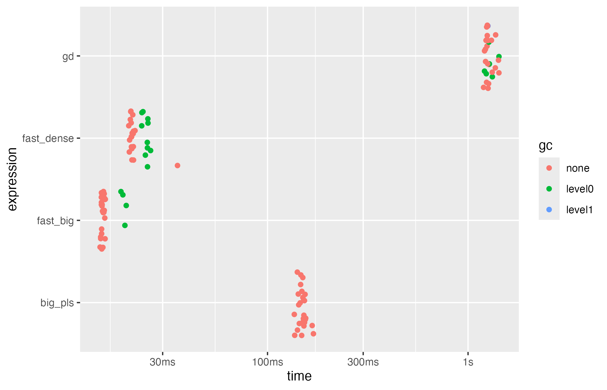
Cleaning up backing files
File-backed matrices can be deleted once the analysis is complete. In
production workflows you typically keep the descriptor
(.desc) file alongside the binary matrix for later
reuse.
Cleaning up
Temporary backing files can be removed after the analysis. In production pipelines you will typically keep the descriptor file alongside the binary data.
if (exists("X_big")) {
  rm(X_big)
  file.remove(file.path(big_dir, "X.bin"))
  file.remove(file.path(big_dir, "X.desc"))
  unlink(big_dir, recursive = TRUE)
}
Further resources
- The introductory vignette demonstrates how to combine the fast backend with the matrix-based modelling functions and deviance residual utilities.
-
vignette("bigPLScox-benchmarking", package = "bigPLScox")provides a reproducible benchmark that includessurvival::coxph()andcoxgpls(). - The help pages (
?big_pls_cox_fast,?big_pls_cox_gd) describe all tuning parameters in detail, includingkeepXfor component-wise sparsity.