Benchmarking bigPLScox
Frédéric Bertrand
Cedric, Cnam, Parisfrederic.bertrand@lecnam.net
2025-11-16
Source:vignettes/bigPLScox-benchmarking.Rmd
bigPLScox-benchmarking.RmdMotivation
The bigPLScox package now provides three distinct
engines for extracting PLS components in Cox regression: the original
matrix-based solver (big_pls_cox), the new Armadillo
backend (big_pls_cox_fast), and the stochastic gradient
descent routine (big_pls_cox_gd). This vignette shows how
to benchmark those implementations against coxgpls() and
the standard survival::coxph() fit.
We rely on the bench package to collect
timing and memory statistics. All chunks are wrapped in the
LOCAL flag so that CRAN builds can skip the heavier
computations.
Simulated data
We reuse the helper dataCox() to generate survival
outcomes with right censoring. Adjust n and p
to stress-test the solvers on larger problems.
set.seed(2024)
sim_design <- dataCox(
  n = 2000,
  lambda = 2,
  rho = 1.5,
  x = matrix(rnorm(2000 * 50), ncol = 50),
  beta = c(1, 3, rep(0, 48)),
  cens.rate = 5
)

cox_data <- list(
  x = as.matrix(sim_design[, -(1:3)]),
  time = sim_design$time,
  status = sim_design$status
)

X_big <- bigmemory::as.big.matrix(cox_data$x)
Running the benchmark
-
Dense matrix scenario – compares the classical
coxgpls()workflow and the dense variants of the big-memory solvers againstsurvival::coxph(). -
Big-memory scenario – evaluates
big_pls_cox_fast()andbig_pls_cox_gd()directly on abig.matrix, illustrating the benefit of the shared-memory interface.
The number of iterations can be increased for more stable measurements when running locally.
Dense matrix comparison
bench_dense <- bench::mark(
  coxgpls = coxgpls(
    cox_data$x,
    cox_data$time,
    cox_data$status,
    ncomp = 5
  ),
  big_pls = big_pls_cox(cox_data$x, cox_data$time, cox_data$status, ncomp = 5),
  big_pls_fast = big_pls_cox_fast(cox_data$x, cox_data$time, cox_data$status, ncomp = 5),
  big_pls_bb = big_pls_cox_gd(X_big, cox_data$time, cox_data$status, ncomp = 5),
  big_pls_gd = big_pls_cox_gd(X_big, cox_data$time, cox_data$status, ncomp = 5, method = "gd"),
  coxph = coxph(Surv(cox_data$time, cox_data$status) ~ cox_data$x, ties = "breslow"),
  iterations = 75,
  check = FALSE
)
bench_dense$expression <- names(bench_dense$expression)
bench_dense[, c("expression", "median", "itr/sec", "mem_alloc")]
#> # A tibble: 6 × 4
#>   expression     median `itr/sec` mem_alloc
#>   <chr>        <bch:tm>     <dbl> <bch:byt>
#> 1 coxgpls       22.01ms     43.6    31.06MB
#> 2 big_pls       144.7ms      6.90    4.34MB
#> 3 big_pls_fast   8.88ms    110.      5.42MB
#> 4 big_pls_bb   394.41ms      2.51    5.71MB
#> 5 big_pls_gd   395.27ms      2.52    5.63MB
#> 6 coxph         28.32ms     35.0    13.39MB
A higher itr/sec value indicates faster throughput. The
fast backend should provide the best compromise between speed and
accuracy in the dense setting.
Big-memory comparison
The next experiment reuses the big.matrix version of the
predictors and adds the SGD solver. Because coxgpls()
requires an in-memory matrix, it is not included in this round.
bench_big <- bench::mark(
  big_pls_fast = big_pls_cox_fast(X_big, cox_data$time, cox_data$status, ncomp = 5),
  big_pls = big_pls_cox(cox_data$x, cox_data$time, cox_data$status, ncomp = 5),
  big_pls_gd = big_pls_cox_gd(X_big, cox_data$time, cox_data$status, ncomp = 5, max_iter = 300),
  iterations = 75,
  check = FALSE
)
bench_big$expression <- names(bench_big$expression)
bench_big[, c("expression", "median", "itr/sec", "mem_alloc")]
#> # A tibble: 3 × 4
#>   expression     median `itr/sec` mem_alloc
#>   <chr>        <bch:tm>     <dbl> <bch:byt>
#> 1 big_pls_fast   7.34ms    136.      3.41MB
#> 2 big_pls      144.98ms      6.93    4.25MB
#> 3 big_pls_gd       66ms     15.0     5.59MB
The classical solver is still run on the dense matrix for reference,
but only the fast and SGD routines operate on the
big.matrix without copying. Expect the fast backend to
dominate runtime while SGD maintains scalability for out-of-memory
workflows.
Visualising the results
bench includes autoplot() and
plot() helpers for visual inspection of the timing
distribution.
plot(bench_dense, type = "jitter")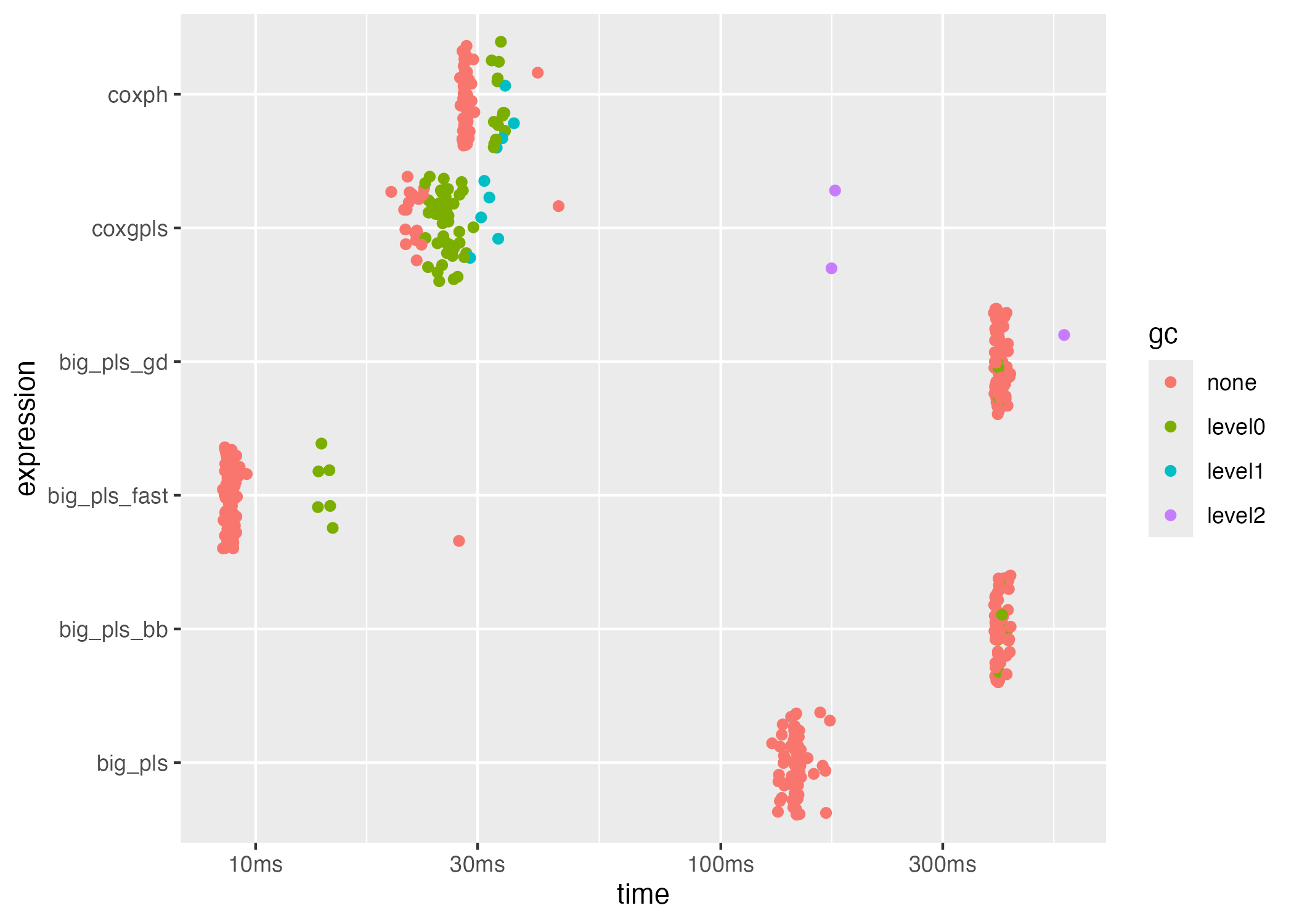
plot(bench_big, type = "jitter")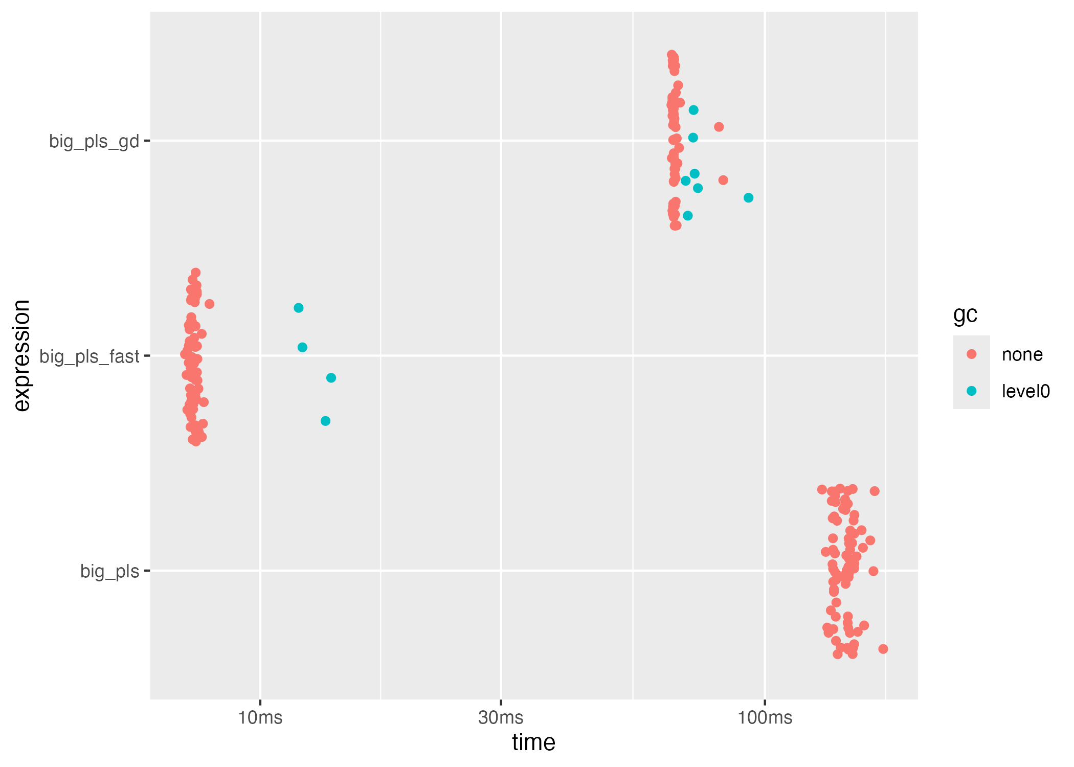
Additional geometries, such as ridge plots, are available via
autoplot(bench_res, type = "jitter").
Exporting benchmark tables
To integrate the benchmark with automated pipelines, store the
results under the inst/benchmarks/ directory. Each run can
include meta-data such as dataset parameters, number of iterations, or
git commit identifiers.
if (!dir.exists("inst/benchmarks/results")) {
  dir.create("inst/benchmarks/results", recursive = TRUE)
}
write.csv(bench_dense[, 1:9], file = "inst/benchmarks/results/benchmark-dense.csv", row.names = FALSE)
write.csv(bench_big[, 1:9], file = "inst/benchmarks/results/benchmark-big.csv", row.names = FALSE)
Additional scripts
The package also ships with standalone scripts under
inst/benchmarks/ that mirror this vignette while exposing
additional configuration points. Run them from the repository root
as:
Rscript inst/benchmarks/cox-benchmark.R
Rscript inst/benchmarks/benchmark_bigPLScox.R
Rscript inst/benchmarks/cox_pls_benchmark.R
Each script accepts environment variables to adjust the problem size
and stores results in inst/benchmarks/results/ with
time-stamped filenames.