Cascade, Selection, Reverse-Engineering and Prediction in Cascade Networks
Frédéric Bertrand and Myriam Maumy-Bertrand
https://doi.org/10.32614/CRAN.package.Cascade
Cascade is a modeling tool allowing gene selection, reverse engineering, and prediction in cascade networks. Jung, N., Bertrand, F., Bahram, S., Vallat, L., and Maumy-Bertrand, M. (2014) https://doi.org/10.1093/bioinformatics/btt705.
The package was presented at the User2014! conference. Jung, N., Bertrand, F., Bahram, S., Vallat, L., and Maumy-Bertrand, M. (2014). “Cascade: a R-package to study, predict and simulate the diffusion of a signal through a temporal genenetwork”, book of abstracts, User2014!, Los Angeles, page 153, https://user2014.r-project.org/abstracts/posters/181_Jung.pdf.
This website and these examples were created by F. Bertrand and M. Maumy-Bertrand.
Installation
You can install the released version of Cascade from CRAN with:
install.packages("Cascade")You can install the development version of Cascade from github with:
devtools::install_github("fbertran/Cascade")Examples
Data management
Import Cascade Data (repeated measurements on several subjects) from the CascadeData package and turn them into a micro array object. The second line makes sure the CascadeData package is installed.
library(Cascade)
if(!require(CascadeData)){install.packages("CascadeData")}
#> Loading required package: CascadeData
data(micro_US)
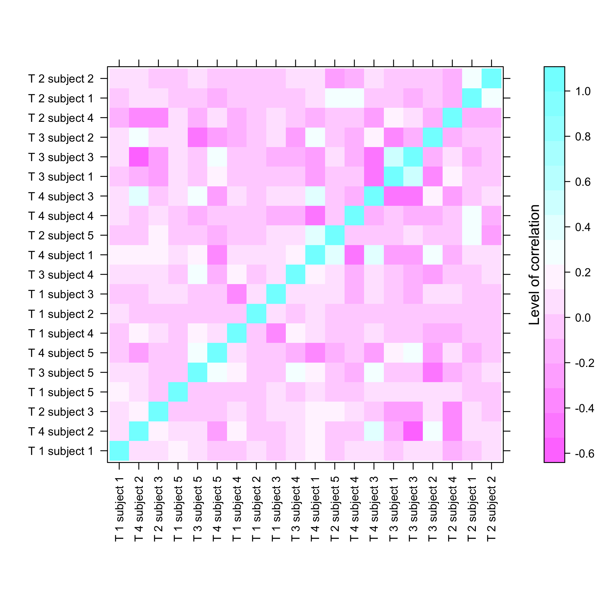
micro_US<-as.micro_array(micro_US,time=c(60,90,210,390),subject=6)Get a summay and plots of the data:
summary(micro_US)
#> Loading required package: cluster
#>    N1_US_T60        N1_US_T90        N1_US_T210       N1_US_T390       N2_US_T60
#>  Min.   :   1.0   Min.   :   1.0   Min.   :   1.0   Min.   :   1.0   Min.   :   1.0
#>  1st Qu.:  19.7   1st Qu.:  18.8   1st Qu.:  15.2   1st Qu.:  20.9   1st Qu.:  18.5
#>  Median :  38.0   Median :  37.2   Median :  34.9   Median :  40.2   Median :  36.9
#>  Mean   : 107.5   Mean   : 106.9   Mean   : 109.6   Mean   : 105.7   Mean   : 110.6
#>  3rd Qu.:  80.6   3rd Qu.:  82.1   3rd Qu.:  82.8   3rd Qu.:  84.8   3rd Qu.:  85.3
#>  Max.   :8587.9   Max.   :8311.7   Max.   :7930.3   Max.   :7841.8   Max.   :7750.3
#>    N2_US_T90        N2_US_T210       N2_US_T390       N3_US_T60        N3_US_T90
#>  Min.   :   1.0   Min.   :   1.0   Min.   :   1.0   Min.   :   1.0   Min.   :   1.0
#>  1st Qu.:  17.1   1st Qu.:  15.8   1st Qu.:  17.7   1st Qu.:  17.3   1st Qu.:  19.5
#>  Median :  36.7   Median :  36.0   Median :  37.4   Median :  34.4   Median :  38.2
#>  Mean   : 102.1   Mean   : 106.8   Mean   : 111.3   Mean   : 101.6   Mean   : 107.1
#>  3rd Qu.:  78.2   3rd Qu.:  83.5   3rd Qu.:  86.4   3rd Qu.:  75.4   3rd Qu.:  82.3
#>  Max.   :8014.3   Max.   :8028.6   Max.   :7498.4   Max.   :8072.2   Max.   :7889.2
#>    N3_US_T210       N3_US_T390       N4_US_T60        N4_US_T90        N4_US_T210
#>  Min.   :   1.0   Min.   :   1.0   Min.   :   1.0   Min.   :   1.0   Min.   :   1.0
#>  1st Qu.:  16.4   1st Qu.:  20.9   1st Qu.:  20.4   1st Qu.:  19.5   1st Qu.:  20.5
#>  Median :  34.7   Median :  41.0   Median :  38.9   Median :  38.5   Median :  39.9
#>  Mean   : 100.3   Mean   : 113.9   Mean   : 113.6   Mean   : 114.8   Mean   : 110.1
#>  3rd Qu.:  76.3   3rd Qu.:  89.2   3rd Qu.:  84.6   3rd Qu.:  86.1   3rd Qu.:  86.8
#>  Max.   :8278.2   Max.   :6856.2   Max.   :9502.3   Max.   :9193.4   Max.   :9436.0
#>    N4_US_T390       N5_US_T60        N5_US_T90        N5_US_T210       N5_US_T390
#>  Min.   :   1.0   Min.   :   1.0   Min.   :   1.0   Min.   :   1.0   Min.   :   1.0
#>  1st Qu.:  19.9   1st Qu.:  16.8   1st Qu.:  18.8   1st Qu.:  19.5   1st Qu.:  19.9
#>  Median :  38.8   Median :  34.5   Median :  36.9   Median :  38.2   Median :  39.0
#>  Mean   : 111.7   Mean   : 111.3   Mean   : 108.0   Mean   : 107.4   Mean   : 109.8
#>  3rd Qu.:  85.4   3rd Qu.:  82.0   3rd Qu.:  81.4   3rd Qu.:  82.4   3rd Qu.:  84.9
#>  Max.   :8771.0   Max.   :8569.3   Max.   :7970.1   Max.   :8371.0   Max.   :7686.5
#>    N6_US_T60        N6_US_T90        N6_US_T210       N6_US_T390
#>  Min.   :   1.0   Min.   :   1.0   Min.   :   1.0   Min.   :   1.0
#>  1st Qu.:  21.1   1st Qu.:  21.5   1st Qu.:  19.9   1st Qu.:  20.2
#>  Median :  40.9   Median :  40.8   Median :  39.1   Median :  39.4
#>  Mean   : 110.1   Mean   : 108.5   Mean   : 112.0   Mean   : 109.5
#>  3rd Qu.:  86.3   3rd Qu.:  85.6   3rd Qu.:  86.3   3rd Qu.:  86.6
#>  Max.   :8241.0   Max.   :8355.0   Max.   :8207.1   Max.   :9520.0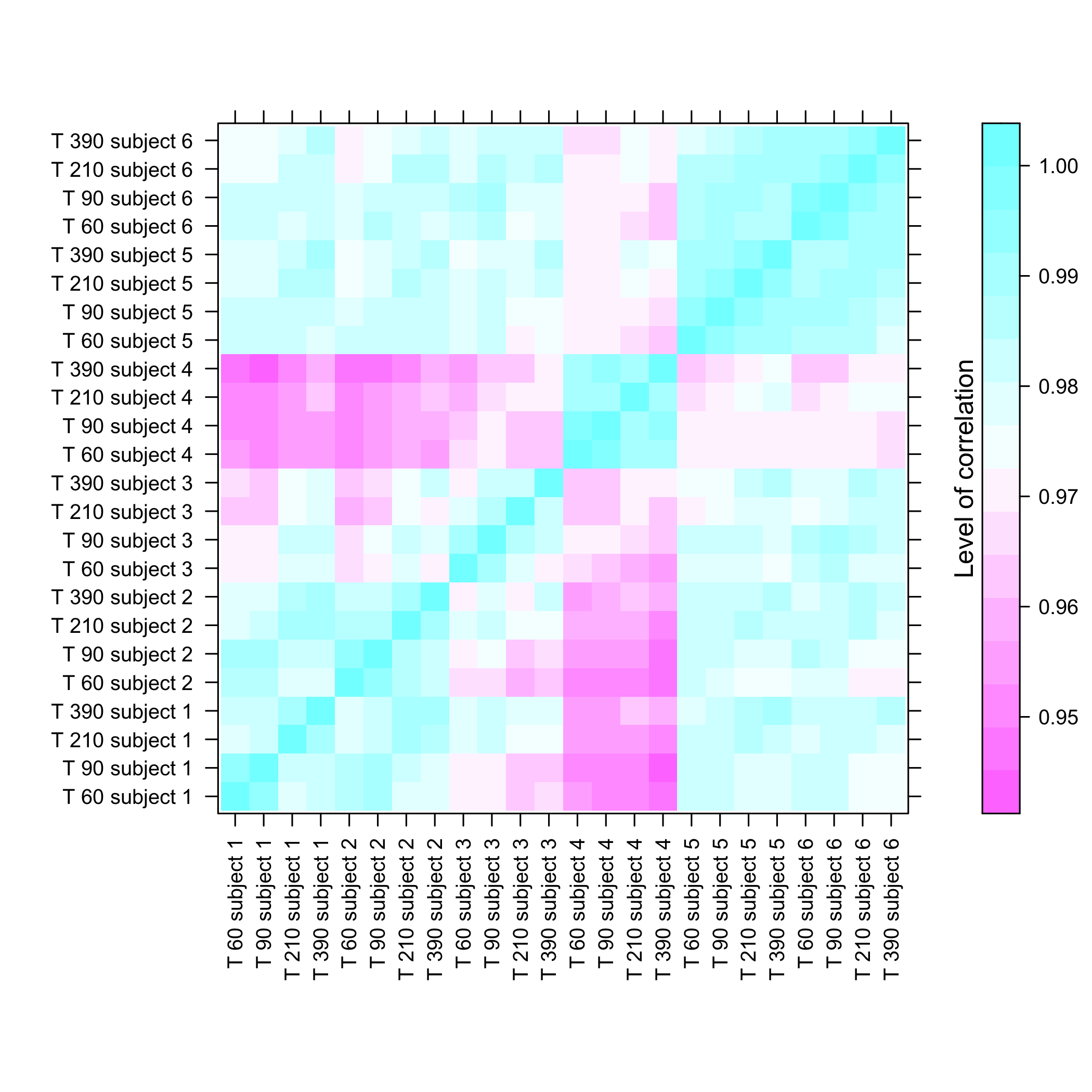
plot of chunk plotmicroarrayclass
plot of chunk plotmicroarrayclass
Gene selection
There are several functions to carry out gene selection before the inference. They are detailed in the package vignette and in the website-only E-MTAB-1475 re-analysis PDF.
Data simulation
Let’s simulate some cascade data and then do some reverse engineering.
We first design the F matrix
T<-4
F<-array(0,c(T-1,T-1,T*(T-1)/2))

for(i in 1:(T*(T-1)/2)){diag(F[,,i])<-1}
F[,,2]<-F[,,2]*0.2
F[2,1,2]<-1
F[3,2,2]<-1
F[,,4]<-F[,,2]*0.3
F[3,1,4]<-1
F[,,5]<-F[,,2]
We set the seed to make the results reproducible and draw a scale free random network.
set.seed(1)
Net<-Cascade::network_random(
  nb=100,
  time_label=rep(1:4,each=25),
  exp=1,
  init=1,
  regul=round(rexp(100,1))+1,
  min_expr=0.1,
  max_expr=2,
  casc.level=0.4
)
Net@F<-F
We simulate gene expression according to the network that was previously drawn
M <- Cascade::gene_expr_simulation(
network=Net,
time_label=rep(1:4,each=25),
subject=5,
level_peak=200)
#> Loading required package: VGAM
#> Loading required package: stats4
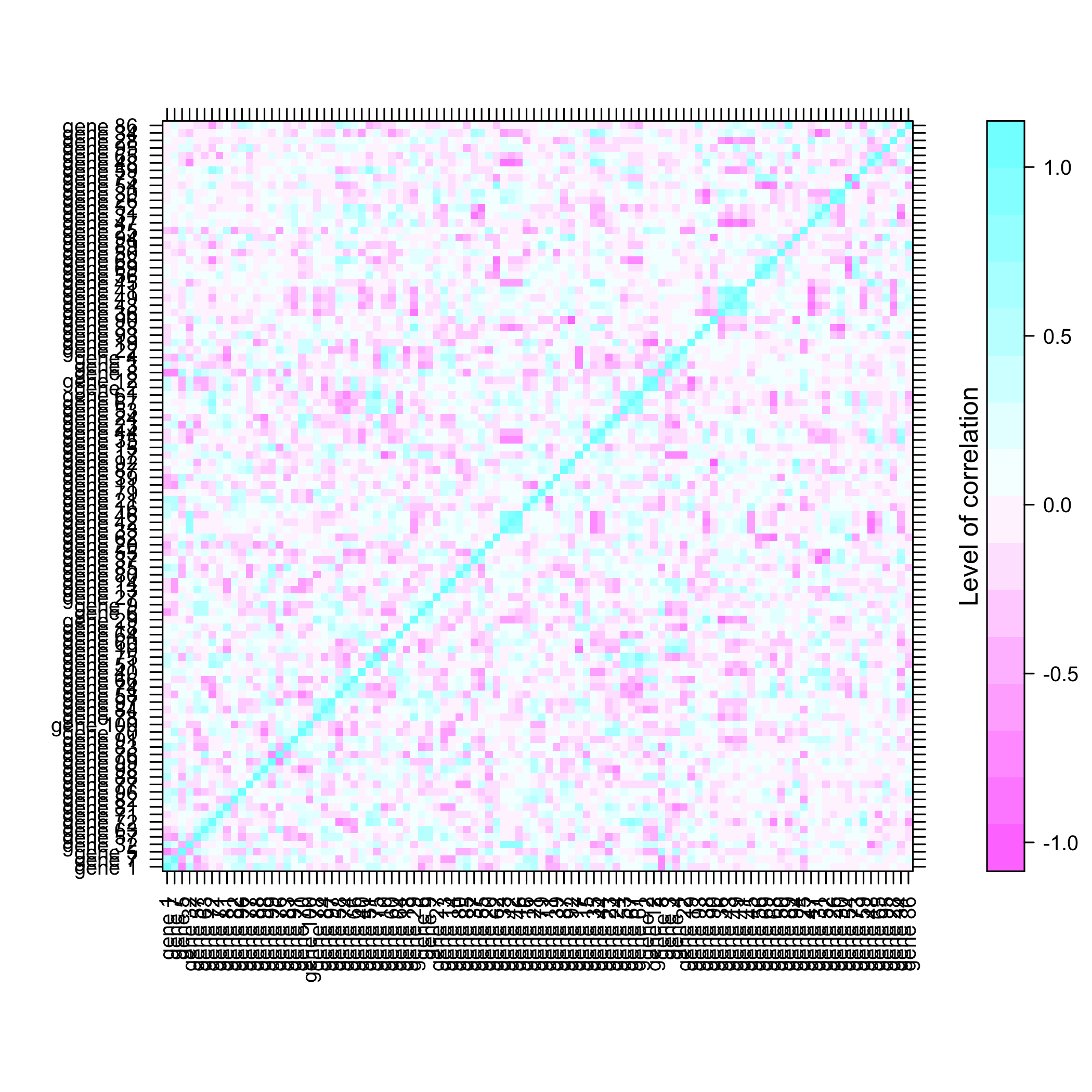
#> Loading required package: splinesGet a summay and plots of the simulated data:
summary(M)
#>  log(S/US) : P1T1   log(S/US) : P1T2    log(S/US) : P1T3    log(S/US) : P1T4
#>  Min.   :-887.428   Min.   :-2060.695   Min.   :-837.5811   Min.   :-2189.33
#>  1st Qu.: -53.644   1st Qu.:  -70.993   1st Qu.: -85.2176   1st Qu.: -115.23
#>  Median :   6.122   Median :    2.206   Median :  -6.6303   Median :  -10.49
#>  Mean   :   3.928   Mean   :   -3.800   Mean   :   0.5563   Mean   :  -75.60
#>  3rd Qu.:  74.894   3rd Qu.:   79.999   3rd Qu.:  71.9501   3rd Qu.:   43.85
#>  Max.   : 747.779   Max.   : 1461.163   Max.   :1279.6850   Max.   :  492.80
#>  log(S/US) : P2T1   log(S/US) : P2T2   log(S/US) : P2T3   log(S/US) : P2T4  log(S/US) : P3T1
#>  Min.   :-431.905   Min.   :-845.072   Min.   :-557.840   Min.   :-660.17   Min.   :-868.834
#>  1st Qu.: -50.282   1st Qu.: -21.668   1st Qu.: -42.958   1st Qu.: -63.34   1st Qu.: -44.656
#>  Median :  -3.782   Median :   2.059   Median :  -2.448   Median : -10.97   Median :   1.839
#>  Mean   :   8.264   Mean   :  18.235   Mean   :  25.290   Mean   :  18.10   Mean   :  -2.150
#>  3rd Qu.:  40.975   3rd Qu.:  40.323   3rd Qu.:  46.573   3rd Qu.:  42.56   3rd Qu.:  55.072
#>  Max.   :1287.819   Max.   : 699.912   Max.   :1754.081   Max.   :1418.99   Max.   : 597.562
#>  log(S/US) : P3T2   log(S/US) : P3T3    log(S/US) : P3T4   log(S/US) : P4T1
#>  Min.   :-953.894   Min.   :-1182.316   Min.   :-1027.24   Min.   :-1012.76
#>  1st Qu.: -59.964   1st Qu.:  -87.170   1st Qu.:  -61.31   1st Qu.:  -33.79
#>  Median :  -1.306   Median :   -2.614   Median :   16.27   Median :   11.57
#>  Mean   :  24.123   Mean   :   10.224   Mean   :   27.52   Mean   :   10.98
#>  3rd Qu.:  78.430   3rd Qu.:   79.246   3rd Qu.:   60.93   3rd Qu.:   74.09
#>  Max.   :1808.233   Max.   : 2761.291   Max.   : 1926.45   Max.   :  891.60
#>  log(S/US) : P4T2   log(S/US) : P4T3   log(S/US) : P4T4   log(S/US) : P5T1
#>  Min.   :-1569.32   Min.   :-577.799   Min.   :-661.083   Min.   :-555.708
#>  1st Qu.: -118.83   1st Qu.: -62.623   1st Qu.: -41.705   1st Qu.: -64.469
#>  Median :  -13.84   Median :  -8.788   Median :  -1.468   Median :   2.697
#>  Mean   :  -63.39   Mean   : -14.803   Mean   :  10.111   Mean   :   9.403
#>  3rd Qu.:   40.22   3rd Qu.:  37.779   3rd Qu.:  67.888   3rd Qu.:  57.251
#>  Max.   :  678.27   Max.   : 430.737   Max.   : 492.723   Max.   : 654.771
#>  log(S/US) : P5T2    log(S/US) : P5T3  log(S/US) : P5T4
#>  Min.   :-1467.268   Min.   :-911.18   Min.   :-621.705
#>  1st Qu.:  -68.769   1st Qu.: -71.66   1st Qu.: -62.466
#>  Median :   -1.565   Median :   1.54   Median :  -5.789
#>  Mean   :    8.180   Mean   :  13.03   Mean   :   7.083
#>  3rd Qu.:   62.256   3rd Qu.:  86.29   3rd Qu.:  62.041
#>  Max.   :  990.550   Max.   :1386.11   Max.   : 689.323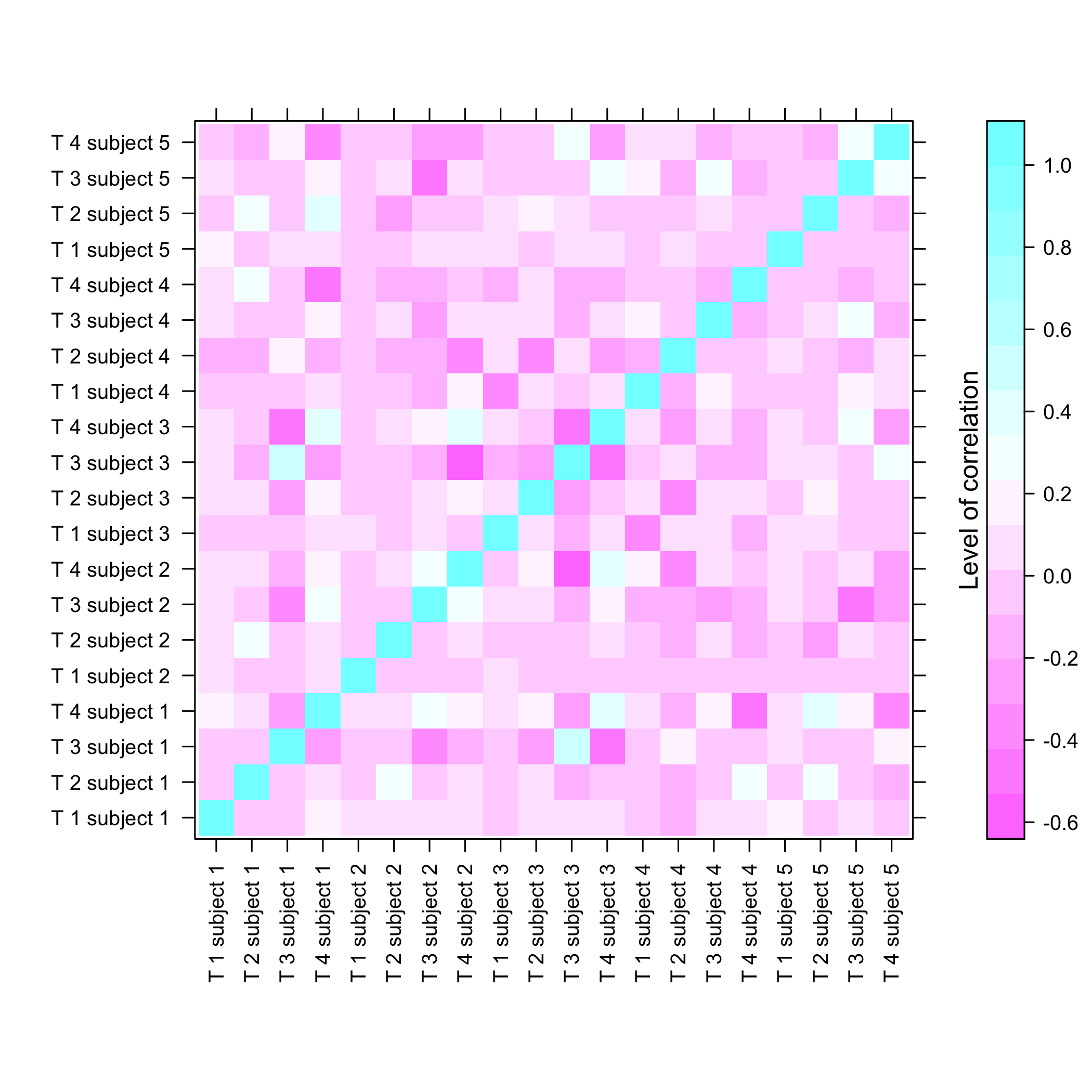
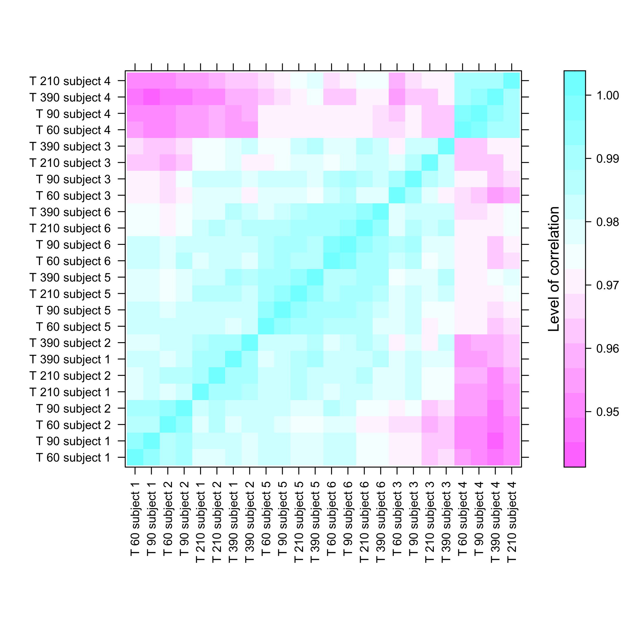
plot of chunk summarysimuldata
plot of chunk summarysimuldata
plot of chunk summarysimuldata
plot(M)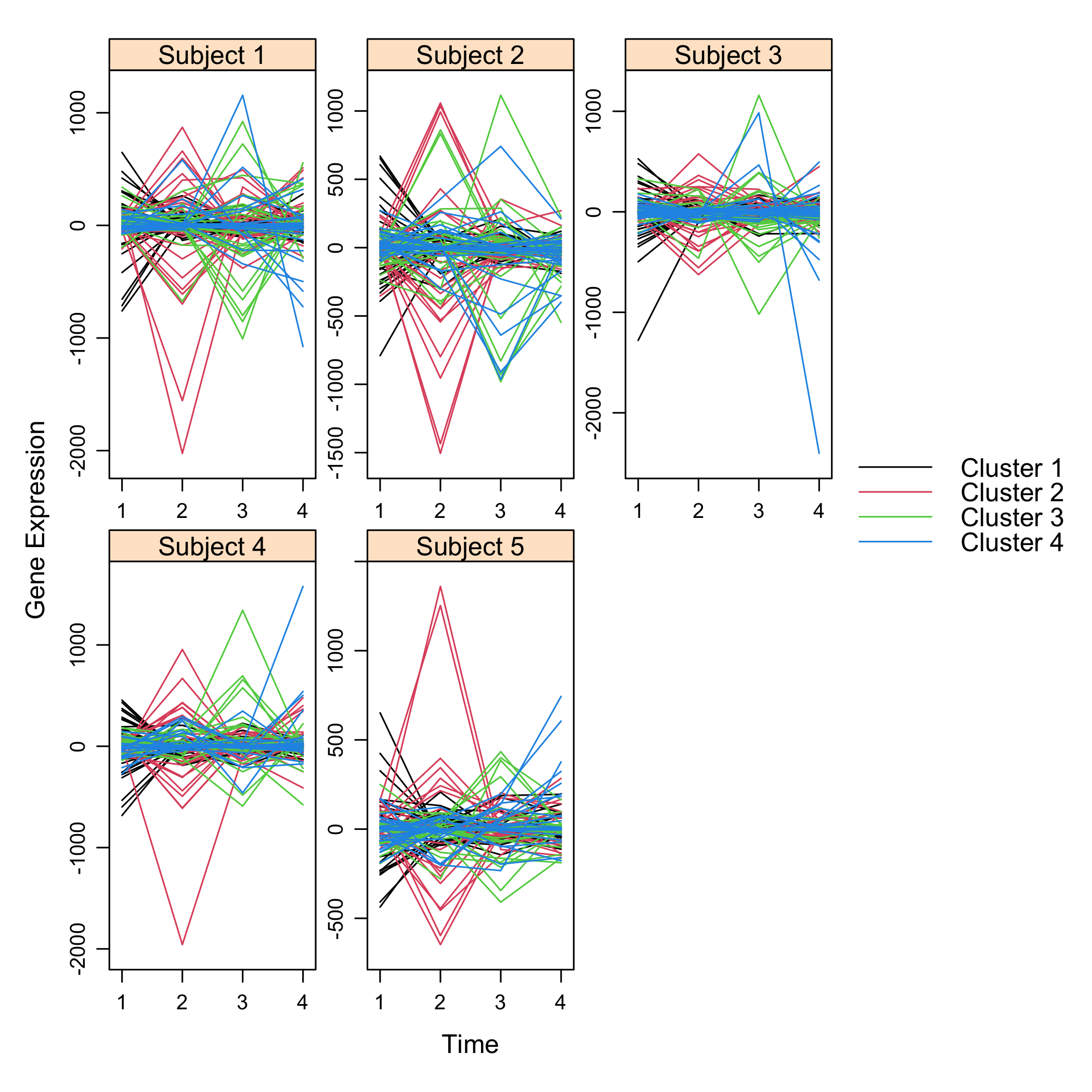
plot of chunk plotsimuldata
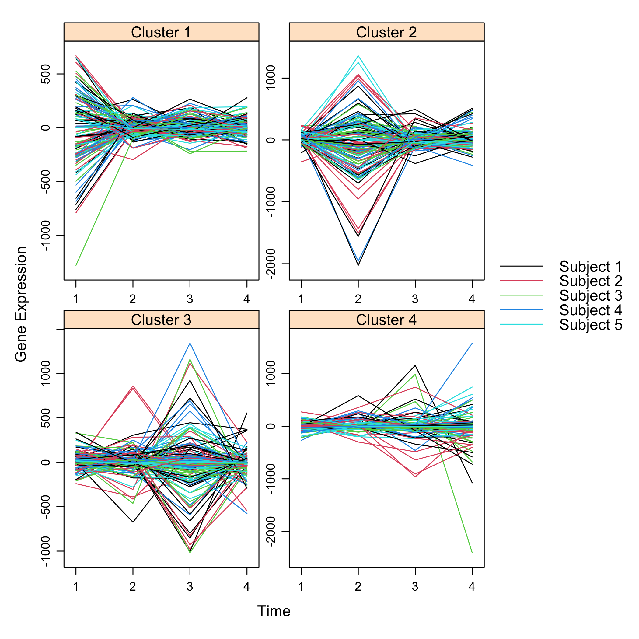
plot of chunk plotsimuldata
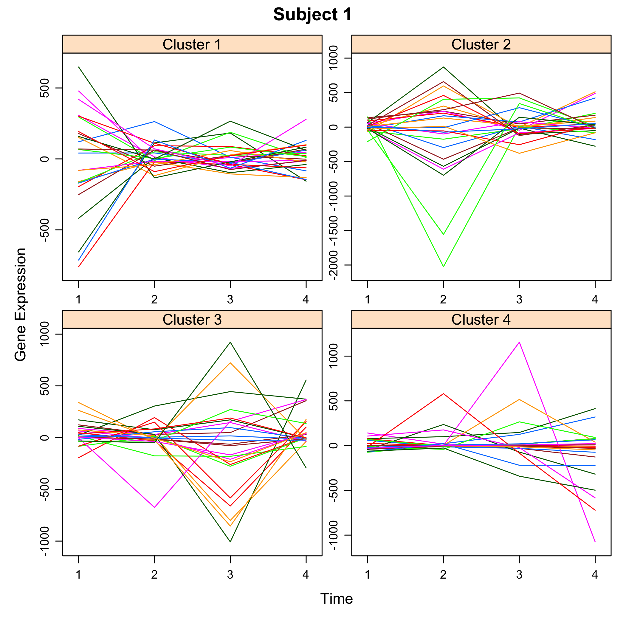
plot of chunk plotsimuldata
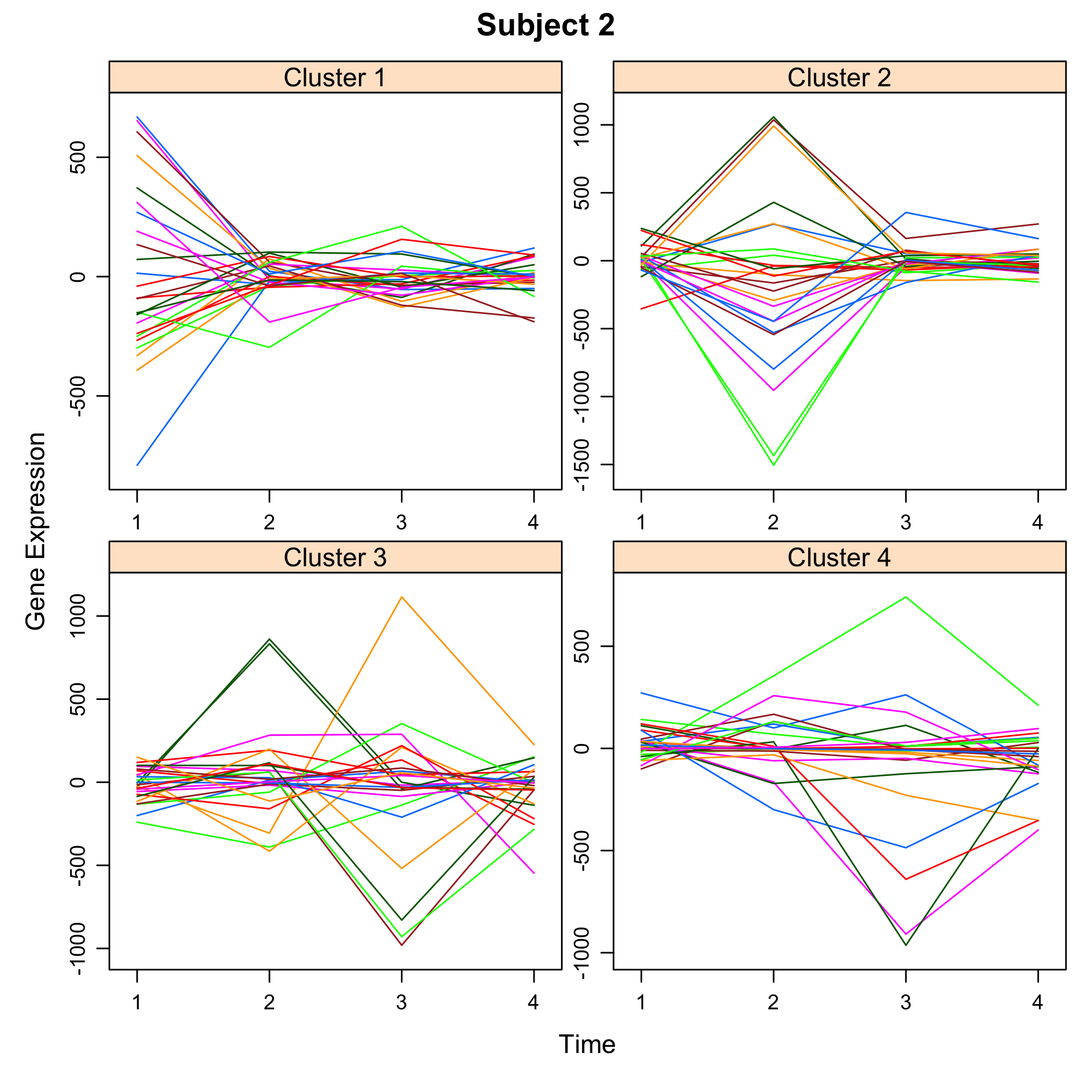
plot of chunk plotsimuldata
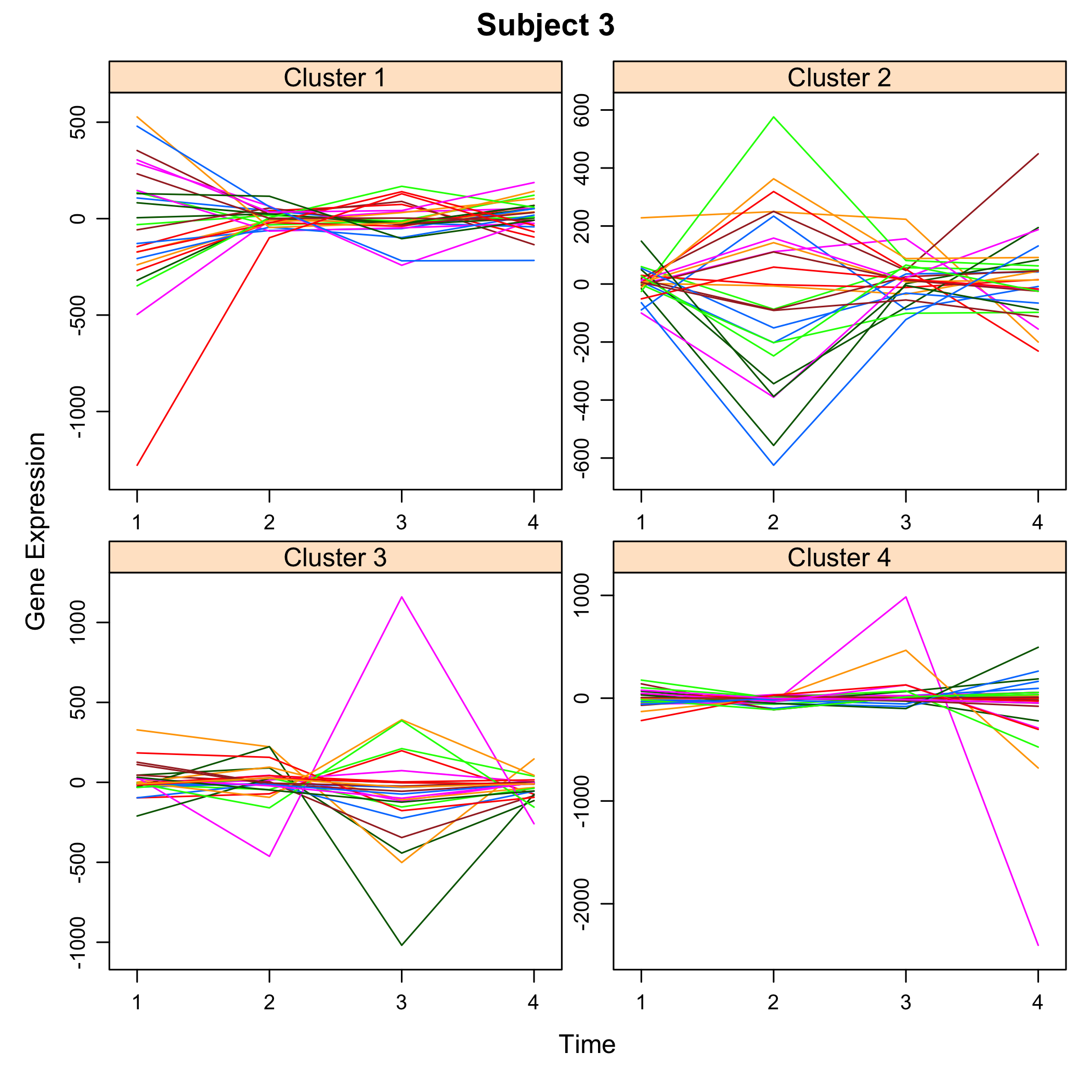
plot of chunk plotsimuldata
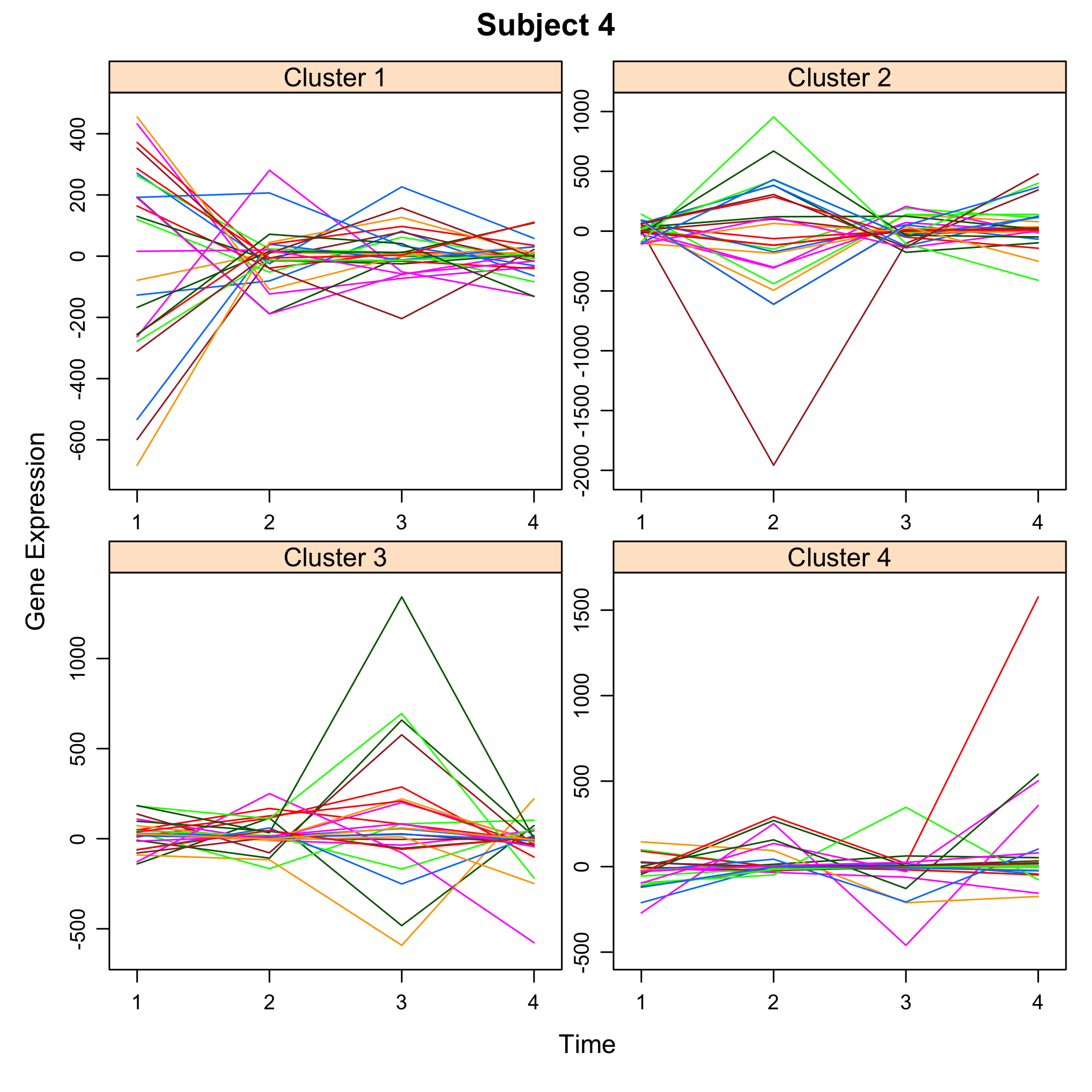
plot of chunk plotsimuldata
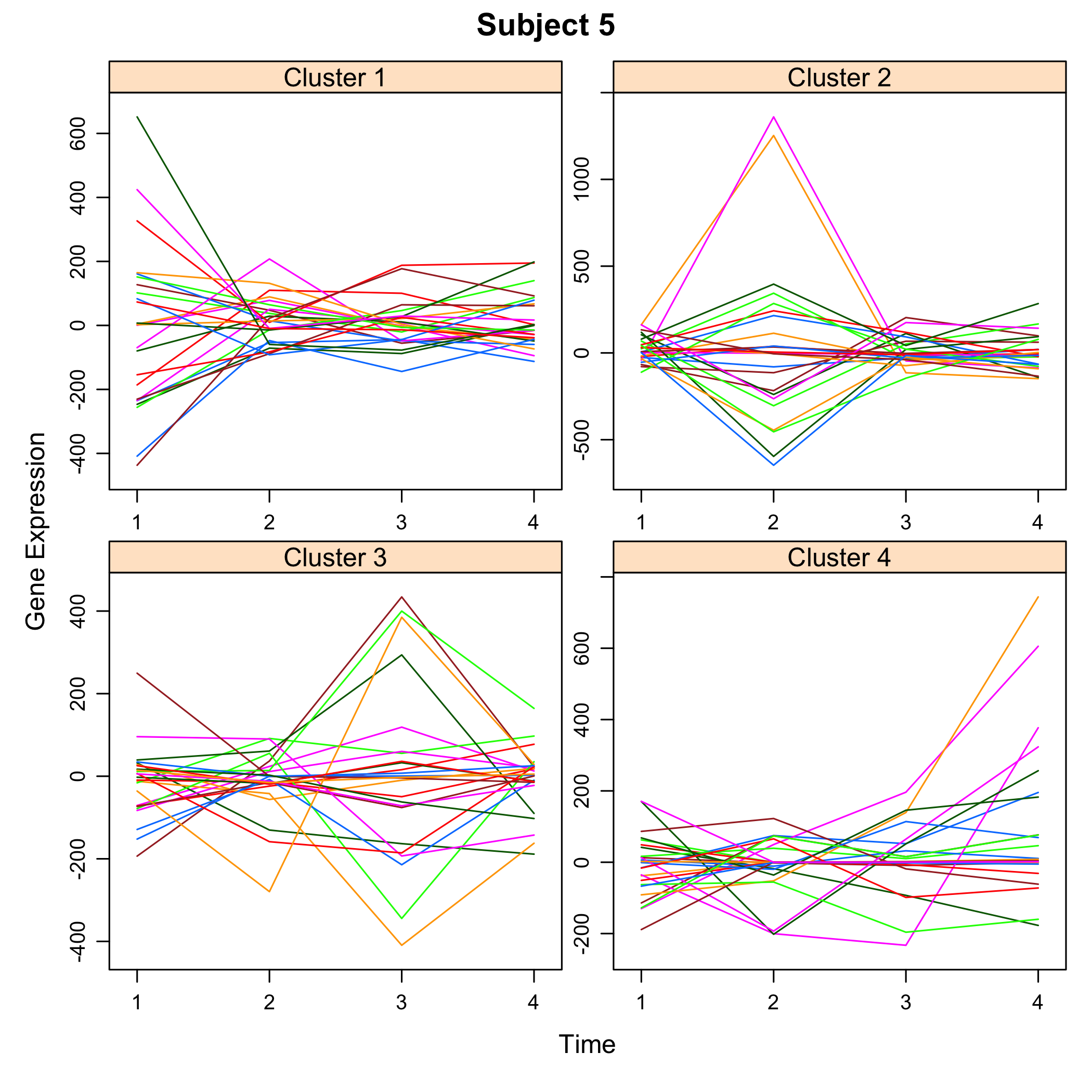
plot of chunk plotsimuldata
Network inference
We infer the new network using subjectwise leave one out cross-validation (all measurement from the same subject are removed from the dataset)
Net_inf_C <- Cascade::inference(M, cv.subjects=TRUE)
#> Loading required package: nnls
#> We are at step :  1
#> The convergence of the network is (L1 norm) : 0.0072
#> We are at step :  2
#> The convergence of the network is (L1 norm) : 0.00139
#> We are at step :  3
#> The convergence of the network is (L1 norm) : 0.00106
#> We are at step :  4
#> The convergence of the network is (L1 norm) : 0.00095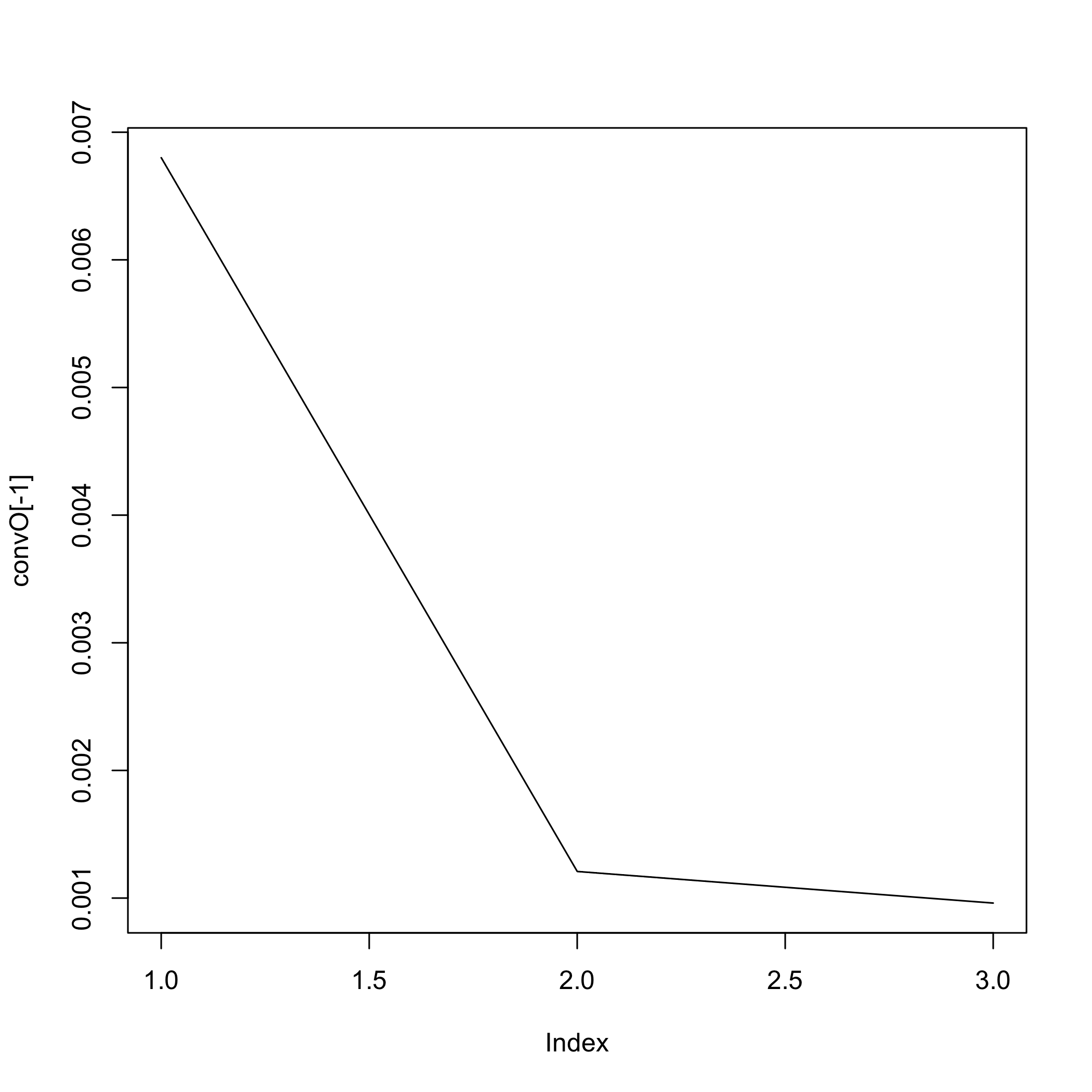
plot of chunk netinf
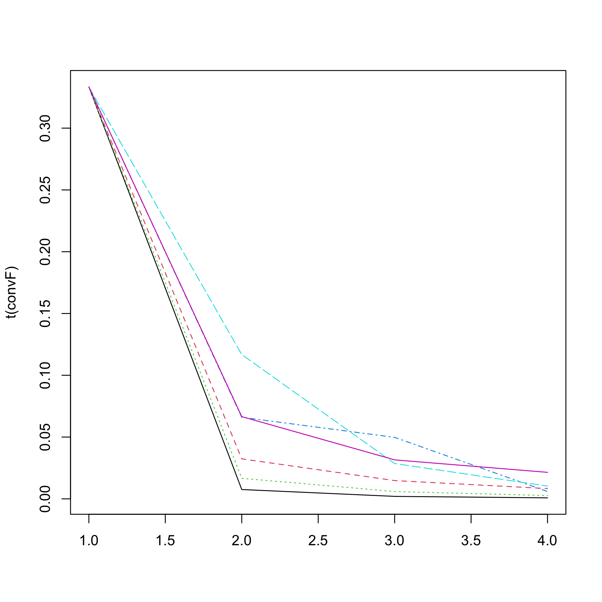
plot of chunk netinf
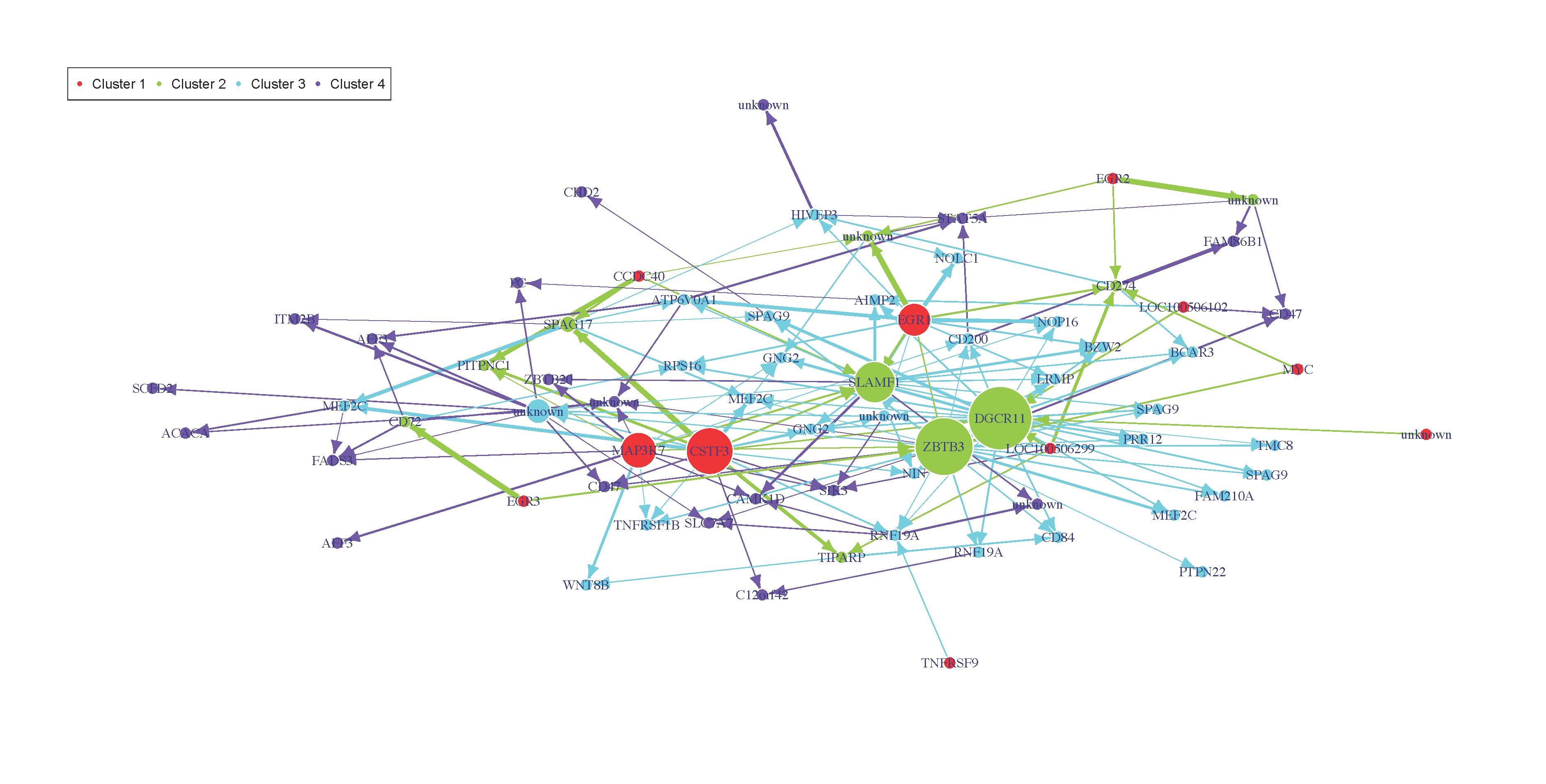
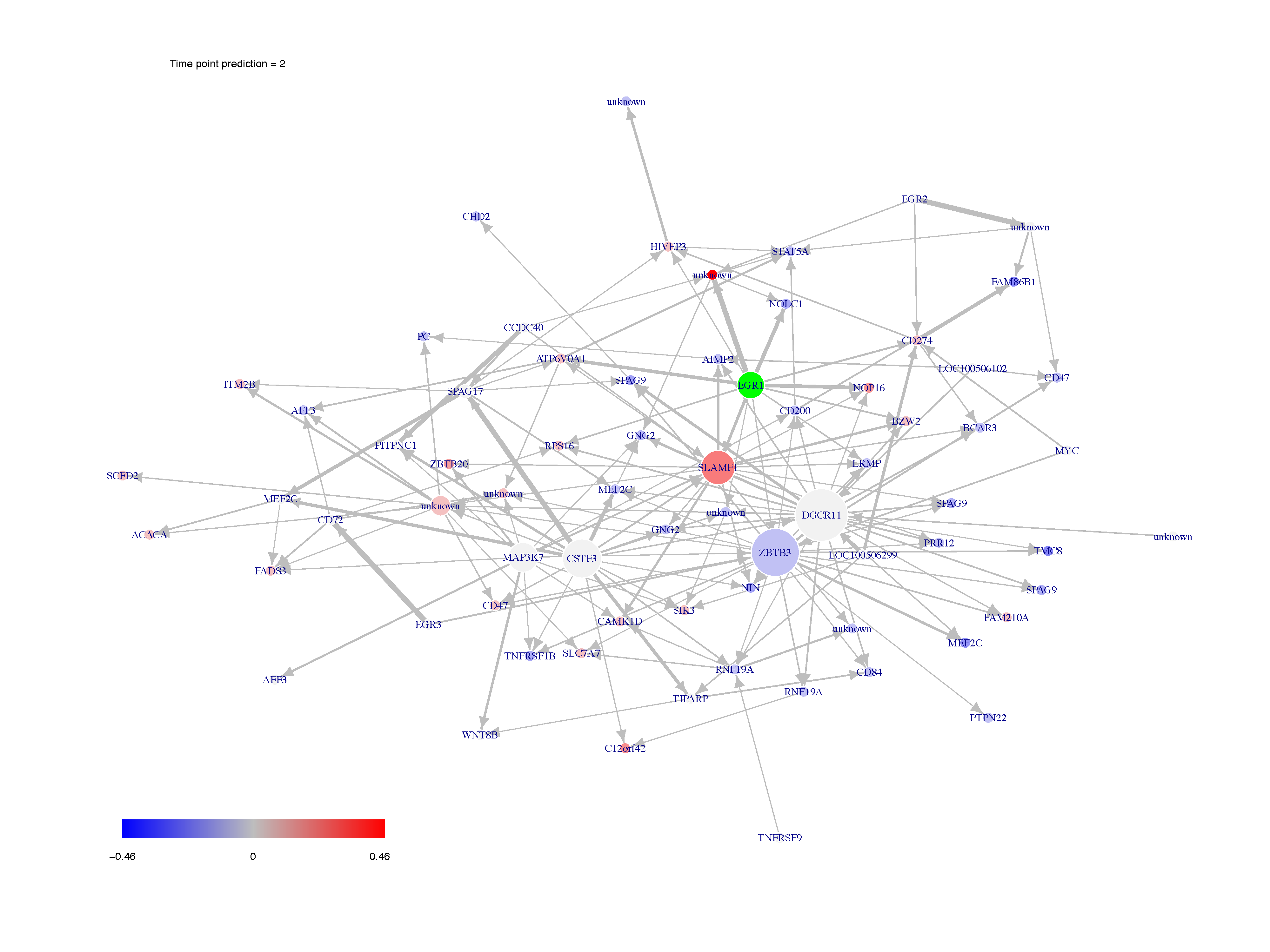
Heatmap of the coefficients of the Omega matrix of the network
stats::heatmap(Net_inf_C@network, Rowv=NA, Colv=NA, scale="none", revC=TRUE)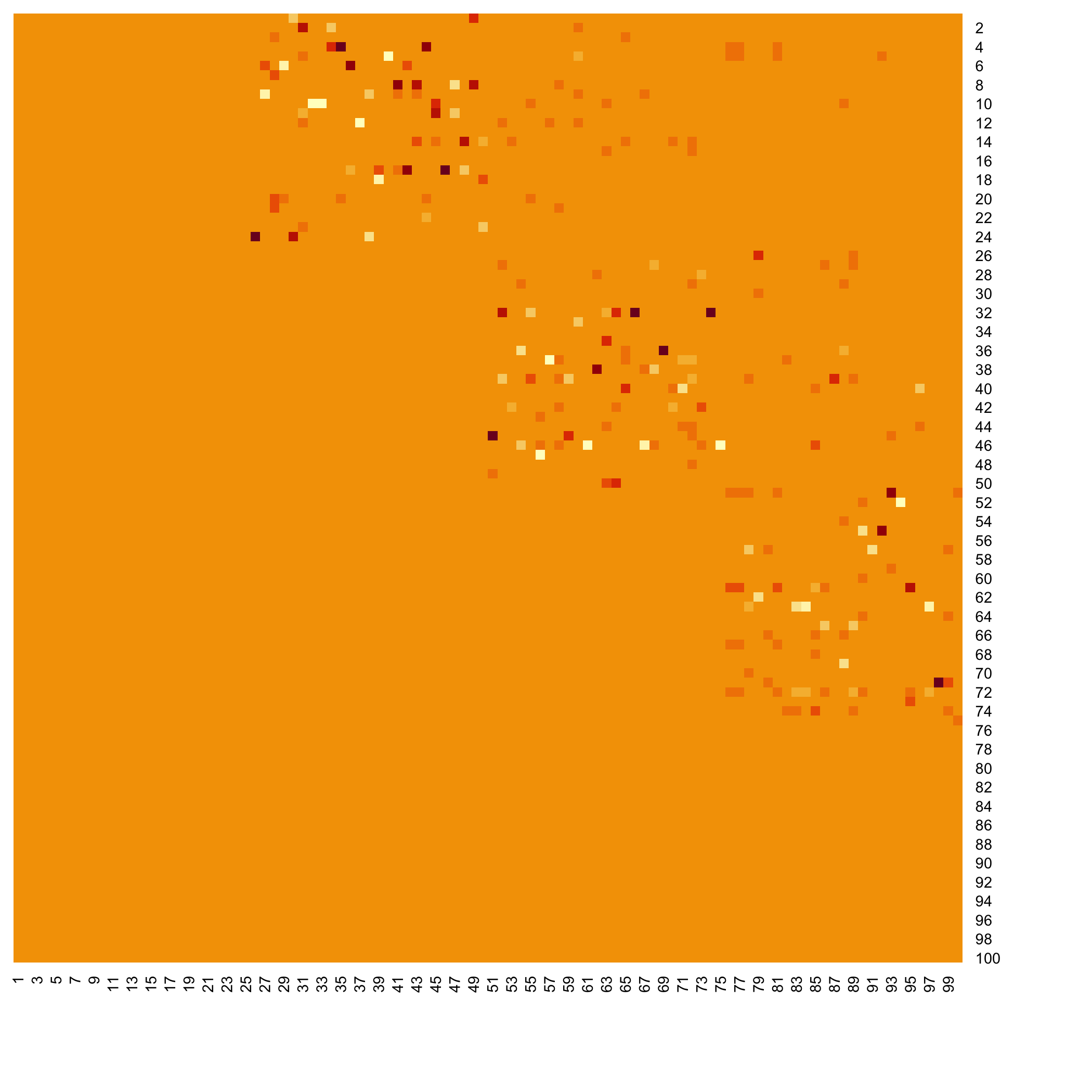
plot of chunk heatresults
###Post inferrence network analysis We switch to data that were derived from the inferrence of a real biological network and try to detect the optimal cutoff value: the best cutoff value for a network to fit a scale free network.
data("network")
set.seed(1)
cutoff(network)
#> [1] "This calculation may be long"
#> [1] "1/10"
#> [1] "2/10"
#> [1] "3/10"
#> [1] "4/10"
#> [1] "5/10"
#> [1] "6/10"
#> [1] "7/10"
#> [1] "8/10"
#> [1] "9/10"
#> [1] "10/10"
#>  [1] 0.000 0.001 0.126 0.112 0.091 0.584 0.885 0.677 0.604 0.363
#> $p.value
#>  [1] 0.000 0.001 0.126 0.112 0.091 0.584 0.885 0.677 0.604 0.363
#>
#> $p.value.inter
#>  [1] 0.0003073808 0.0222769859 0.0521597921 0.0819131661
#>  [5] 0.1859011443 0.5539131661 0.8106723719 0.7795175496
#>  [9] 0.6267996116 0.3396322205
#>
#> $sequence
#>  [1] 0.00000000 0.04444444 0.08888889 0.13333333 0.17777778
#>  [6] 0.22222222 0.26666667 0.31111111 0.35555556 0.40000000
Analyze the network with a cutoff set to the previouly found 0.14 optimal value.
analyze_network(network,nv=0.14)
#>    node betweenness degree    output  closeness
#> 1     1           0      3 0.8133348 16.4471148
#> 2     2           0      3 0.8884602  7.9547696
#> 3     3           0      1 0.1749376 10.0055952
#> 4     4           0      3 0.5159878 11.4854812
#> 5     5           0      0 0.0000000  0.0000000
#> 6     6           0     13 3.5794097 25.6388630
#> 7     7           0      4 0.9685114  7.0356510
#> 8     8           0      0 0.0000000  0.0000000
#> 9     9           0      0 0.0000000  0.0000000
#> 10   10           3      2 0.6047036  3.0439695
#> 11   11          31     10 1.9146802  8.2263869
#> 12   12           1      1 0.2056836  0.8489352
#> 13   13          97     19 3.7578360 18.6066356
#> 14   14           0      0 0.0000000  0.0000000
#> 15   15           0      0 0.0000000  0.0000000
#> 16   16           0      0 0.0000000  0.0000000
#> 17   17           2      2 0.3985715  1.6450577
#> 18   18           9      1 0.1408025  0.5811461
#> 19   19           0      0 0.0000000  0.0000000
#> 20   20           0      0 0.0000000  0.0000000
#> 21   21           0      0 0.0000000  0.0000000
#> 22   22           0      0 0.0000000  0.0000000
#> 23   23           0      0 0.0000000  0.0000000
#> 24   24           0      0 0.0000000  0.0000000
#> 25   25           0      0 0.0000000  0.0000000
#> 26   26           0      0 0.0000000  0.0000000
#> 27   27           0      0 0.0000000  0.0000000
#> 28   28           9      2 0.3786198  1.5627095
#> 29   29           0      0 0.0000000  0.0000000
#> 30   30          28      6 1.1216028  4.6292854
#> 31   31           0      0 0.0000000  0.0000000
#> 32   32           0      0 0.0000000  0.0000000
#> 33   33           0      0 0.0000000  0.0000000
#> 34   34           3      1 0.1988608  0.8207750
#> 35   35           0      0 0.0000000  0.0000000
#> 36   36           0      0 0.0000000  0.0000000
#> 37   37           0      0 0.0000000  0.0000000
#> 38   38           0      0 0.0000000  0.0000000
#> 39   39           0      0 0.0000000  0.0000000
#> 40   40           0      0 0.0000000  0.0000000
#> 41   41           0      0 0.0000000  0.0000000
#> 42   42           0      0 0.0000000  0.0000000
#> 43   43           0      0 0.0000000  0.0000000
#> 44   44           0      0 0.0000000  0.0000000
#> 45   45           0      0 0.0000000  0.0000000
#> 46   46           0      0 0.0000000  0.0000000
#> 47   47           0      0 0.0000000  0.0000000
#> 48   48           0      0 0.0000000  0.0000000
#> 49   49           0      0 0.0000000  0.0000000
#> 50   50           0      0 0.0000000  0.0000000
#> 51   51           0      0 0.0000000  0.0000000
#> 52   52           0      0 0.0000000  0.0000000
#> 53   53           0      0 0.0000000  0.0000000
#> 54   54           0      0 0.0000000  0.0000000
#> 55   55           0     10 3.2277268 22.2234874
#> 56   56          13      3 0.7360000  3.5063367
#> 57   57           0      0 0.0000000  0.0000000
#> 58   58           1      1 0.2291004  0.9455855
#> 59   59           0      0 0.0000000  0.0000000
#> 60   60           0      2 0.3955933  7.4313822
#> 61   61           0      3 1.2813639  7.0435303
#> 62   62           0      0 0.0000000  0.0000000
#> 63   63           0      0 0.0000000  0.0000000
#> 64   64           2      2 0.3878745  1.6009071
#> 65   65           0      2 1.2169141 10.8093303
#> 66   66           5      1 0.3016614  1.2450723
#> 67   67           3      3 0.5958934  2.4594808
#> 68   68           0      0 0.0000000  0.0000000
#> 69   69           0      0 0.0000000  0.0000000
#> 70   70           0      0 0.0000000  0.0000000
#> 71   71          26      8 1.6479964  6.8019142
#> 72   72           0      0 0.0000000  0.0000000
#> 73   73           0      0 0.0000000  0.0000000
#> 74   74           0      0 0.0000000  0.0000000