Sobol4R: Sobol indices for a stochastic process model
Frédéric Bertrand
Cedric, Cnam, Parisfrederic.bertrand@lecnam.net
2025-11-26
Source:vignettes/Sobol4R_vignette_process.Rmd
Sobol4R_vignette_process.RmdIntroduction
This vignette presents a simple stochastic process model in which the quantity of interest is the time needed to reach a given number of successes. The model is defined at the level of individual units and is driven by exponential and Bernoulli random variables.
The goal is to compute Sobol indices for this model when the distributional parameters are uncertain.
Process model
The elementary unit is implemented by sobol4r_one_unit.
The individual level model sobol4r_process_indiv aggregates
units up to a target number of successes.
Sobol4R:::one_unit(
  lambda1 = 1 / 60,
  lambda2 = 1 / 1012,
  lambda3 = 1 / 72,
  p1      = 0.18,
  p2      = 0.5
)
#> [1] 0.000000000 0.005804484 0.000000000
process_fun_indiv(
  X_indiv = c(
    lambda1 = 1 / 60,
    lambda2 = 1 / 1012,
    lambda3 = 1 / 72,
    p1      = 0.18,
    p2      = 0.5
  ),
  M = 50
)
#> [1] 7.957008
Design for distributional parameters
We build two designs X1 and X2 for the
uncertain distributional parameters, which are interpreted row wise by
the process model.
n <- 200

draw_params <- function(n) {
  data.frame(t(replicate(
    n,
    c(
      1 / runif(1, min = 20,  max = 100),
      1 / runif(1, min = 24,  max = 2000),
      1 / runif(1, min = 24,  max = 120),
      runif(1,  min = 0.05, max = 0.3),
      runif(1,  min = 0.3,  max = 0.7)
    )
  )))
}

X1 <- draw_params(n)
X2 <- draw_params(n)
gensol_proc <- sobol4r_design(
  X1    = X1,
  X2    = X2,
  order = 2,
  nboot = 100
)
gensol_proc_s2007 <- sensitivity::sobol2007(
  model=NULL,
  X1    = X1,
  X2    = X2,
  nboot = 100
)
Sobol indices based on a single trajectory
Yproc_1 <- process_fun_row_wise(gensol_proc$X, M = 50)
Yproc_s2007 <- process_fun_row_wise(gensol_proc_s2007$X, M = 50)
print(xproc_1)
#>
#> Call:
#> sensitivity::sobol(model = NULL, X1 = X1, X2 = X2, order = order,     nboot = nboot)
#>
#> Model runs: 3200
#>
#> Sobol indices
#>         original        bias std. error   min. c.i. max. c.i.
#> X1     0.7294194  0.00049123  0.2513380  0.27950991 1.2084699
#> X2     0.3004787  0.01349792  0.2051145 -0.13490482 0.7166861
#> X3     0.2957471  0.01592217  0.2070449 -0.12608586 0.7172049
#> X4     0.4559113  0.03160123  0.1843086 -0.05077489 0.7265388
#> X5     0.2830712  0.01852571  0.1932263 -0.14990173 0.6354526
#> X1*X2 -0.3343066 -0.01325800  0.2249487 -0.78555566 0.1210838
#> X1*X3 -0.3561771 -0.01217180  0.2339348 -0.83051127 0.0965282
#> X1*X4 -0.2413266 -0.02257892  0.2991820 -0.83675497 0.4176541
#> X1*X5 -0.3770702 -0.02718860  0.2554472 -0.80990616 0.1701954
#> X2*X3 -0.3276111 -0.01458000  0.2181632 -0.77870900 0.1372350
#> X2*X4 -0.3314252 -0.01645722  0.2121561 -0.77316732 0.1201331
#> X2*X5 -0.2658610 -0.01500736  0.1969157 -0.64640003 0.1536311
#> X3*X4 -0.3287880 -0.02359720  0.2308614 -0.80781454 0.1625249
#> X3*X5 -0.3408354 -0.01815007  0.2109176 -0.77419315 0.1081724
#> X4*X5 -0.2694589 -0.03160427  0.2357108 -0.77577433 0.2093851
Sobol4R::autoplot(xproc_1, ncol = 1)
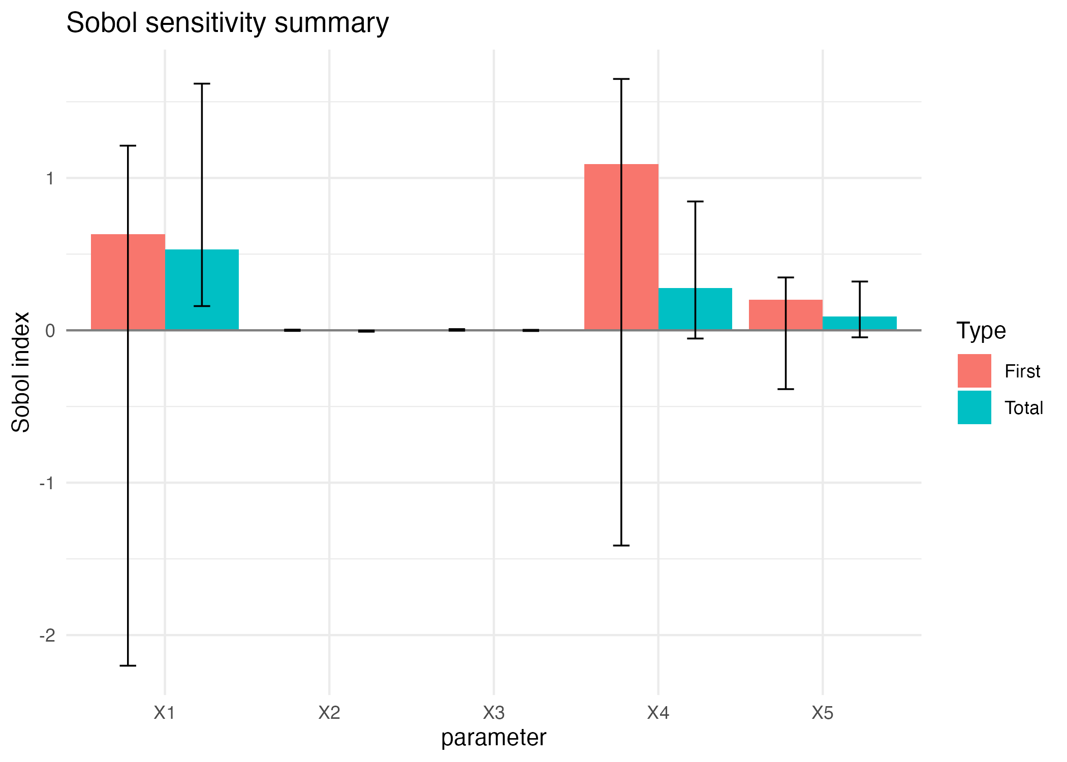
print(xproc_s2007)
#>
#> Call:
#> sensitivity::sobol2007(model = NULL, X1 = X1, X2 = X2, nboot = 100)
#>
#> Model runs: 1400
#>
#> First order indices:
#>      original         bias std. error   min. c.i. max. c.i.
#> X1 0.78059654  0.026966701 0.41791588 -0.36770953 1.2991697
#> X2 0.06366468 -0.003512076 0.04786715 -0.03869592 0.1654700
#> X3 0.01459135  0.004726172 0.05483269 -0.12825874 0.1130782
#> X4 1.19394885  0.043419466 0.48734070 -0.22090457 1.8623500
#> X5 0.25311374  0.007218066 0.17030381 -0.21513710 0.4998055
#>
#> Total indices:
#>         original         bias std. error  min. c.i. max. c.i.
#> X1  0.5496354427 -0.013111901 0.15117956  0.3141528 0.9015871
#> X2 -0.0564200705  0.017020644 0.12324393 -0.3508908 0.1377340
#> X3  0.0005891851  0.002411750 0.08555174 -0.1771735 0.1720782
#> X4  0.2799643974  0.003049293 0.18861940 -0.1241736 0.7284894
#> X5  0.1145422977  0.019339225 0.16685350 -0.1760436 0.5269174
Sobol4R::autoplot(xproc_s2007)
Sobol indices based on a quantity of interest
Instead of relying on a single trajectory, we can define a quantity
of interest for each parameter vector, for instance the mean time to
reach the target number of successes. This is implemented by
sobol4r_process_qoi.
Yproc_2 <- process_fun_mean_to_M(gensol_proc$X, M = 50)
xproc_2 <- tell(gensol_proc, Yproc_2)
print(xproc_2)
#>
#> Call:
#> sensitivity::sobol(model = NULL, X1 = X1, X2 = X2, order = order,     nboot = nboot)
#>
#> Model runs: 3200
#>
#> Sobol indices
#>         original         bias std. error  min. c.i. max. c.i.
#> X1     0.6826528  0.005126550  0.2480252  0.1485698 1.1439030
#> X2     0.3176581  0.010674480  0.2562279 -0.3787595 0.7167677
#> X3     0.3258947  0.010487470  0.2590476 -0.3617596 0.7387714
#> X4     0.4393571  0.030845038  0.1988659 -0.1607166 0.7436733
#> X5     0.3392149  0.024193718  0.2463190 -0.3970669 0.6981421
#> X1*X2 -0.2939788 -0.015211110  0.2582148 -0.6842354 0.4084324
#> X1*X3 -0.2888089 -0.013018485  0.2550826 -0.6937357 0.3831304
#> X1*X4 -0.1505352 -0.044984037  0.3261704 -0.6404235 0.8520856
#> X1*X5 -0.2639892 -0.017353912  0.2690282 -0.7042267 0.5228493
#> X2*X3 -0.3326051 -0.009993783  0.2634304 -0.7466524 0.3659032
#> X2*X4 -0.3162005 -0.013351054  0.2591504 -0.7103273 0.3887268
#> X2*X5 -0.3336627 -0.011750294  0.2602581 -0.7391448 0.3635950
#> X3*X4 -0.3331674 -0.014007668  0.2625429 -0.7420036 0.3590781
#> X3*X5 -0.3592000 -0.011309098  0.2699409 -0.7894881 0.3693090
#> X4*X5 -0.2954550 -0.014510084  0.2700965 -0.7333147 0.4146974
Sobol4R::autoplot(xproc_2, ncol = 1)
Qoi Mean
res_sobol_mean <- sobol4r_qoi_indices(
  model = process_fun_row_wise,
  X1      = X1,
  X2      = X2,
  qoi_fun = base::mean,
  nrep    = 1000,
  order   = 2,
  nboot   = 20,
  M       = 50,
  type  = "sobol"
)
print(res_sobol_mean)
#>
#> Call:
#> sensitivity::sobol(model = NULL, X1 = X1, X2 = X2, order = order,     nboot = nboot)
#>
#> Model runs: 3200
#>
#> Sobol indices
#>         original        bias std. error   min. c.i. max. c.i.
#> X1     0.6805953  0.06579726  0.2915201 -0.05931977 0.9930548
#> X2     0.3008859  0.06145805  0.3413658 -0.88236392 0.7524947
#> X3     0.3006451  0.06103511  0.3406389 -0.88045781 0.7527655
#> X4     0.4360898  0.03680453  0.2247240 -0.15502002 0.8089744
#> X5     0.3148892  0.03602053  0.2789583 -0.64795152 0.6789437
#> X1*X2 -0.2975536 -0.06198502  0.3420717 -0.74813653 0.8906007
#> X1*X3 -0.3005069 -0.06094272  0.3412032 -0.75336817 0.8830056
#> X1*X4 -0.2010131 -0.08869790  0.2984828 -0.65529321 0.6336699
#> X1*X5 -0.2684205 -0.04696034  0.3456393 -0.78315616 0.8685432
#> X2*X3 -0.3009403 -0.06143294  0.3414768 -0.75223685 0.8835731
#> X2*X4 -0.3014412 -0.06123680  0.3413067 -0.75356381 0.8799221
#> X2*X5 -0.3009248 -0.06137610  0.3412708 -0.75236900 0.8822591
#> X3*X4 -0.3007574 -0.06061473  0.3404276 -0.75275578 0.8777120
#> X3*X5 -0.3019780 -0.06057977  0.3402788 -0.75334627 0.8785105
#> X4*X5 -0.2758623 -0.05966790  0.3633708 -0.75818965 1.0111646
Sobol4R::autoplot(res_sobol_mean, ncol = 1)
res_sobol2007_mean <- sobol4r_qoi_indices(
  model = process_fun_row_wise,
  X1      = X1,
  X2      = X2,
  qoi_fun = base::mean,
  nrep    = 1000,
  nboot   = 20,
  M       = 50,
  type  = "sobol2007"
)
print(res_sobol2007_mean)
#>
#> Call:
#> sensitivity::sobol2007(model = NULL, X1 = X1, X2 = X2, nboot = nboot)
#>
#> Model runs: 1400
#>
#> First order indices:
#>        original          bias   std. error     min. c.i.   max. c.i.
#> X1 0.6274357275  1.933040e-02 0.3441016539 -0.3398362883 1.103774781
#> X2 0.0008242769 -2.249057e-04 0.0015807319 -0.0023759905 0.004029758
#> X3 0.0021233184  9.417988e-05 0.0009865046  0.0004880764 0.003496689
#> X4 1.0975117805 -5.208604e-02 0.4394763913 -0.1537345782 1.689410619
#> X5 0.2019065056  9.312831e-03 0.1290530635 -0.2074654193 0.335771533
#>
#> Total indices:
#>        original          bias  std. error    min. c.i.    max. c.i.
#> X1  0.532059804  5.967415e-03 0.128915919  0.280135144  0.713385892
#> X2 -0.002240093  5.903650e-04 0.002408428 -0.007549059  0.002190784
#> X3 -0.006024882 -2.606107e-05 0.001853114 -0.010555671 -0.003532359
#> X4  0.276844920  3.518714e-02 0.201009767 -0.041162140  0.677923530
#> X5  0.089923585  9.174677e-03 0.145860899 -0.167883254  0.362529675
Sobol4R::autoplot(res_sobol2007_mean)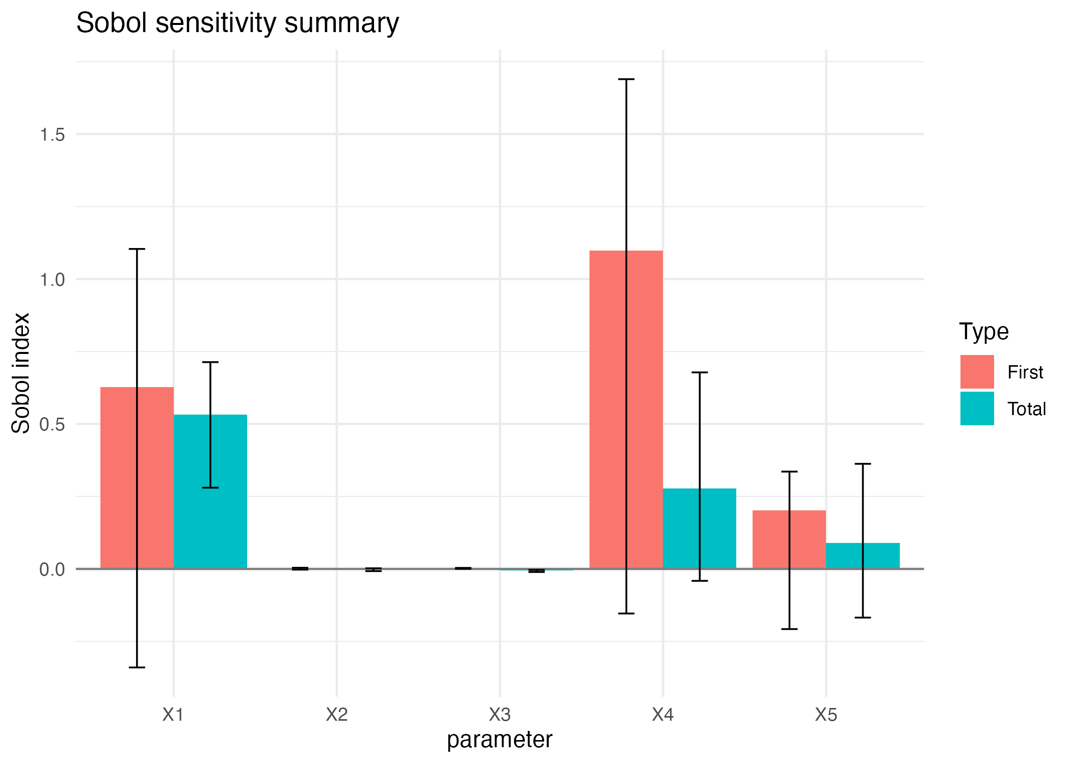
Qoi Median
res_sobol_median <- sobol4r_qoi_indices(
  model = process_fun_row_wise,
  X1      = X1,
  X2      = X2,
  qoi_fun = stats::median,
  nrep    = 1000,
  order   = 2,
  nboot   = 20,
  M       = 50,
  type    = "sobol"
)
print(res_sobol_median)
#>
#> Call:
#> sensitivity::sobol(model = NULL, X1 = X1, X2 = X2, order = order,     nboot = nboot)
#>
#> Model runs: 3200
#>
#> Sobol indices
#>         original        bias std. error   min. c.i.  max. c.i.
#> X1     0.6838808  0.01427035  0.2499123  0.17006140 1.03003325
#> X2     0.3014619 -0.05854112  0.2068283 -0.04052554 0.65190549
#> X3     0.3040197 -0.05880441  0.2075153 -0.04033192 0.65456686
#> X4     0.4366072 -0.05765811  0.1426287  0.23387014 0.76553497
#> X5     0.3140690 -0.05265660  0.1807080 -0.04093714 0.63087985
#> X1*X2 -0.3070862  0.05959257  0.2079712 -0.66535925 0.03393730
#> X1*X3 -0.3086261  0.05931663  0.2088386 -0.66287107 0.03655093
#> X1*X4 -0.2024409  0.04294745  0.2480517 -0.60097971 0.25398309
#> X1*X5 -0.2691735  0.07250931  0.2014423 -0.63794781 0.06340764
#> X2*X3 -0.3053052  0.05812156  0.2080119 -0.65361007 0.04307241
#> X2*X4 -0.3019594  0.05897805  0.2063651 -0.65378906 0.03870985
#> X2*X5 -0.3021756  0.05851692  0.2072934 -0.65305783 0.04274170
#> X3*X4 -0.3040339  0.05914784  0.2074400 -0.65703109 0.04036785
#> X3*X5 -0.3030301  0.05775997  0.2085067 -0.65238401 0.04808432
#> X4*X5 -0.2749564  0.05147778  0.2196955 -0.63229036 0.10439382
Sobol4R::autoplot(res_sobol_median, ncol = 1)
res_sobol2007_median <- sobol4r_qoi_indices(
  model = process_fun_row_wise,
  X1      = X1,
  X2      = X2,
  qoi_fun = stats::median,
  nrep    = 1000,
  nboot   = 20,
  M       = 50,
  type    = "sobol2007"
)
print(res_sobol2007_median)
#>
#> Call:
#> sensitivity::sobol2007(model = NULL, X1 = X1, X2 = X2, nboot = nboot)
#>
#> Model runs: 1400
#>
#> First order indices:
#>       original         bias  std. error    min. c.i.   max. c.i.
#> X1 0.631136293 0.3518396529 0.892602725 -2.201165768 1.211889780
#> X2 0.001271101 0.0009124744 0.002369515 -0.003964884 0.004411122
#> X3 0.002570528 0.0004359652 0.002344942 -0.002486295 0.007781618
#> X4 1.090728028 0.2415061369 0.732729339 -1.412514753 1.649640844
#> X5 0.201706947 0.0879264537 0.206641333 -0.386047563 0.346867853
#>
#> Total indices:
#>        original          bias  std. error    min. c.i.    max. c.i.
#> X1  0.531523669 -0.0729994672 0.331167907  0.158962886  1.618870406
#> X2 -0.004751456 -0.0001029459 0.002192107 -0.009031976 -0.001528655
#> X3 -0.002405476 -0.0006439060 0.002279635 -0.004597536  0.002993045
#> X4  0.278546795 -0.1029523197 0.255775665 -0.053865835  0.845646247
#> X5  0.089823287 -0.0084978131 0.093193129 -0.046021882  0.320166482
Sobol4R::autoplot(res_sobol2007_median)