Exploring Sobol indices and randomness with Sobol4R

Context and non random case

Test case: the non monotonic Sobol g function.

The method of Sobol requires two samples. In the reference case there are eight variables, all following the uniform distribution on [0,1].

n <- 50000
p <- 8
X1_1 <- data.frame(matrix(runif(p * n), nrow = n))
X2_1 <- data.frame(matrix(runif(p * n), nrow = n))

set.seed(4669)
gensol1 <- sobol4r_design(
  X1    = X1_1,
  X2    = X2_1,
  order = 2,
  nboot = 100
)

Y1 <- sobol_g_function(gensol1$X)
x1 <- sensitivity::tell(gensol1, Y1)

print(x1)
#> 
#> Call:
#> sensitivity::sobol(model = NULL, X1 = X1, X2 = X2, order = order,     nboot = nboot)
#> 
#> Model runs: 1850000 
#> 
#> Sobol indices
#>           original          bias  std. error    min. c.i.   max. c.i.
#> X1     0.716687957 -0.0007506201 0.007568642  0.704904998 0.734553717
#> X2     0.194138905  0.0018867840 0.008564673  0.176095217 0.207794424
#> X3     0.039178654  0.0013086099 0.009998164  0.019745844 0.059106198
#> X4     0.021909025  0.0015247991 0.009997951  0.003894803 0.041782281
#> X5     0.015876506  0.0013797535 0.009862420 -0.001965988 0.034335093
#> X6     0.015293824  0.0013589275 0.009871009 -0.002615684 0.033739384
#> X7     0.015450641  0.0013999418 0.009830706 -0.002197353 0.033817776
#> X8     0.015562056  0.0013687406 0.009844287 -0.002136192 0.033977458
#> X1*X2  0.041788726 -0.0014391412 0.011696617  0.023128993 0.063640694
#> X1*X3 -0.004937621 -0.0013769088 0.010189394 -0.024998516 0.014213072
#> X1*X4 -0.012526950 -0.0013056630 0.009838578 -0.031409287 0.005563374
#> X1*X5 -0.015425841 -0.0013720959 0.009837824 -0.033839972 0.002382693
#> X1*X6 -0.015508012 -0.0013759868 0.009852874 -0.034022908 0.002314938
#> X1*X7 -0.015453405 -0.0013748933 0.009855058 -0.033903651 0.002345500
#> X1*X8 -0.015234479 -0.0013635338 0.009858249 -0.033729585 0.002642363
#> X2*X3 -0.013781931 -0.0013834260 0.010083740 -0.033094752 0.004612368
#> X2*X4 -0.015114158 -0.0013642767 0.009859457 -0.032856631 0.002174834
#> X2*X5 -0.015325040 -0.0013700765 0.009842260 -0.033751492 0.002433855
#> X2*X6 -0.015426095 -0.0013705172 0.009860968 -0.033834409 0.002380184
#> X2*X7 -0.015498387 -0.0013703407 0.009857096 -0.033982323 0.002313440
#> X2*X8 -0.015379072 -0.0013761200 0.009857861 -0.033867275 0.002451179
#> X3*X4 -0.015295522 -0.0013685560 0.009851201 -0.033647569 0.002410603
#> X3*X5 -0.015392995 -0.0013743295 0.009853136 -0.033839855 0.002394021
#> X3*X6 -0.015422268 -0.0013763614 0.009854233 -0.033896298 0.002353486
#> X3*X7 -0.015404783 -0.0013725225 0.009855842 -0.033875858 0.002390569
#> X3*X8 -0.015399436 -0.0013759847 0.009851659 -0.033854408 0.002385207
#> X4*X5 -0.015401983 -0.0013752728 0.009854837 -0.033854638 0.002388293
#> X4*X6 -0.015406381 -0.0013761556 0.009853664 -0.033862786 0.002374637
#> X4*X7 -0.015397762 -0.0013744247 0.009853931 -0.033855040 0.002387126
#> X4*X8 -0.015416027 -0.0013755172 0.009852570 -0.033867548 0.002359941
#> X5*X6 -0.015409013 -0.0013758226 0.009853706 -0.033857819 0.002379628
#> X5*X7 -0.015408390 -0.0013757150 0.009853857 -0.033858408 0.002379668
#> X5*X8 -0.015407502 -0.0013757377 0.009853607 -0.033855348 0.002380915
#> X6*X7 -0.015409257 -0.0013758069 0.009853620 -0.033857453 0.002378392
#> X6*X8 -0.015406676 -0.0013758051 0.009853758 -0.033853956 0.002382148
#> X7*X8 -0.015408348 -0.0013757551 0.009853896 -0.033858828 0.002380025
Sobol4R::autoplot(x1, ncol = 1)

ex1_results <- sobol_example_g_deterministic()
print(ex1_results)
#> 
#> Call:
#> sensitivity::sobol(model = NULL, X1 = X1, X2 = X2, order = order,     nboot = nboot)
#> 
#> Model runs: 1850000 
#> 
#> Sobol indices
#>            original          bias  std. error    min. c.i.  max. c.i.
#> X1     0.7245997507  1.318649e-04 0.006865099  0.711583661 0.73855259
#> X2     0.1852412158 -6.379462e-04 0.009725422  0.163919891 0.20792418
#> X3     0.0321041221 -3.943572e-04 0.009939738  0.012874359 0.05265936
#> X4     0.0150373622 -3.716233e-04 0.009571601 -0.002765501 0.03471590
#> X5     0.0073639355 -5.240577e-04 0.009690646 -0.010879190 0.02837068
#> X6     0.0073304377 -5.140176e-04 0.009697496 -0.010964117 0.02838793
#> X7     0.0072934310 -5.369366e-04 0.009679297 -0.010989042 0.02830642
#> X8     0.0070625492 -5.292390e-04 0.009661789 -0.010934969 0.02789333
#> X1*X2  0.0459216617  8.939108e-05 0.010932749  0.026094148 0.06869013
#> X1*X3 -0.0006600465  6.814819e-04 0.010010933 -0.022980303 0.01844932
#> X1*X4 -0.0056037444  4.901684e-04 0.009860488 -0.026644889 0.01263961
#> X1*X5 -0.0070363484  5.187023e-04 0.009676301 -0.027999214 0.01120229
#> X1*X6 -0.0071411552  5.319393e-04 0.009690812 -0.028192638 0.01110205
#> X1*X7 -0.0072518362  5.303046e-04 0.009672163 -0.028265971 0.01093724
#> X1*X8 -0.0070777721  5.186929e-04 0.009676468 -0.028051234 0.01119551
#> X2*X3 -0.0051274794  5.279125e-04 0.009702252 -0.026495177 0.01365939
#> X2*X4 -0.0060860874  5.210190e-04 0.009681757 -0.027207071 0.01195456
#> X2*X5 -0.0071063957  5.147476e-04 0.009680715 -0.028066083 0.01115791
#> X2*X6 -0.0071163219  5.256144e-04 0.009679855 -0.028098511 0.01109647
#> X2*X7 -0.0070620281  5.299198e-04 0.009678650 -0.028017158 0.01116083
#> X2*X8 -0.0071567767  5.166541e-04 0.009686683 -0.028157933 0.01108562
#> X3*X4 -0.0073116996  5.314332e-04 0.009671714 -0.028275534 0.01102687
#> X3*X5 -0.0071206761  5.265249e-04 0.009682280 -0.028100457 0.01114042
#> X3*X6 -0.0071350887  5.241734e-04 0.009680955 -0.028110685 0.01112504
#> X3*X7 -0.0071632203  5.264482e-04 0.009681046 -0.028151981 0.01111060
#> X3*X8 -0.0071109279  5.241054e-04 0.009682418 -0.028109093 0.01117038
#> X4*X5 -0.0071437469  5.248274e-04 0.009679986 -0.028127750 0.01111732
#> X4*X6 -0.0071379129  5.276560e-04 0.009680886 -0.028127090 0.01112126
#> X4*X7 -0.0071596546  5.255998e-04 0.009681341 -0.028150168 0.01109302
#> X4*X8 -0.0071300368  5.260610e-04 0.009682262 -0.028120750 0.01114550
#> X5*X6 -0.0071348129  5.263360e-04 0.009681340 -0.028121862 0.01112445
#> X5*X7 -0.0071382804  5.262539e-04 0.009681217 -0.028124558 0.01111832
#> X5*X8 -0.0071340327  5.262561e-04 0.009681110 -0.028120227 0.01112288
#> X6*X7 -0.0071357204  5.261516e-04 0.009681295 -0.028121656 0.01112018
#> X6*X8 -0.0071339651  5.264348e-04 0.009681123 -0.028121004 0.01112360
#> X7*X8 -0.0071370385  5.263348e-04 0.009681299 -0.028124733 0.01112035

Sobol4R::autoplot(ex1_results, ncol = 1)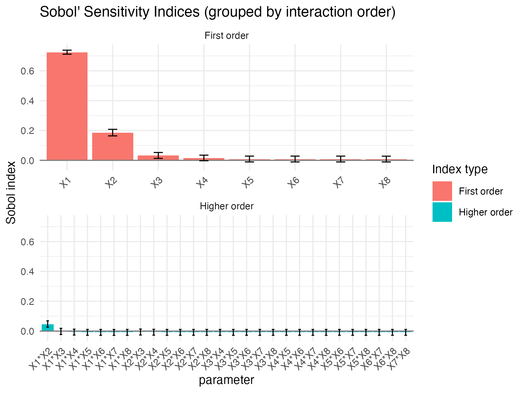

Sobol and randomness I: random effect on output variable

Generate data

n <- 50000
X1_r1 <- data.frame(
  C1 = runif(n),
  C2 = runif(n)
)
X2_r1 <- data.frame(
  C1 = runif(n),
  C2 = runif(n)
)

Three settings, two input variables

The deterministic model is sobol4r_g2. The noisy version with Gaussian noise N(0,1) is sobol4r_g2_noise_const. The quantity of interest based on the mean over replications is sobol4r_g2_noise_const_qoi_mean.

set.seed(4669)
gensol2 <- sobol4r_design(
  X1    = X1_r1,
  X2    = X2_r1,
  order = 2,
  nboot = 100
)

Y2 <- sobol_g2_function(gensol2$X)
Y3 <- sobol_g2_additive_noise(gensol2$X)
Y4 <- sobol_g2_qoi_mean(gensol2$X, nrep = 1000)

x2 <- sensitivity::tell(gensol2, Y2)
x3 <- sensitivity::tell(gensol2, Y3)
x4 <- sensitivity::tell(gensol2, Y4)

print(x2)
#> 
#> Call:
#> sensitivity::sobol(model = NULL, X1 = X1, X2 = X2, order = order,     nboot = nboot)
#> 
#> Model runs: 200000 
#> 
#> Sobol indices
#>         original          bias  std. error  min. c.i. max. c.i.
#> C1    0.75294715 -0.0020757531 0.007497918 0.73603349 0.7706049
#> C2    0.18208419  0.0001224554 0.008328073 0.16719942 0.1969894
#> C1*C2 0.06501351  0.0019533167 0.011592068 0.04149586 0.0885798
print(x3)
#> 
#> Call:
#> sensitivity::sobol(model = NULL, X1 = X1, X2 = X2, order = order,     nboot = nboot)
#> 
#> Model runs: 200000 
#> 
#> Sobol indices
#>         original          bias  std. error    min. c.i.  max. c.i.
#> C1    0.22708608 -0.0009503416 0.006064791  0.218750413 0.24323115
#> C2    0.05211258 -0.0005337665 0.006966395  0.038261623 0.06533689
#> C1*C2 0.01970182  0.0010269693 0.010380381 -0.002741708 0.04006086
print(x4)
#> 
#> Call:
#> sensitivity::sobol(model = NULL, X1 = X1, X2 = X2, order = order,     nboot = nboot)
#> 
#> Model runs: 200000 
#> 
#> Sobol indices
#>         original          bias  std. error  min. c.i. max. c.i.
#> C1    0.75117252  0.0008298031 0.006824511 0.73696397 0.7653366
#> C2    0.18248043 -0.0017367430 0.009332159 0.16508020 0.2069736
#> C1*C2 0.06457593  0.0009315934 0.012032118 0.04010188 0.0874222

Sobol4R::autoplot(x2)

Sobol4R::autoplot(x3)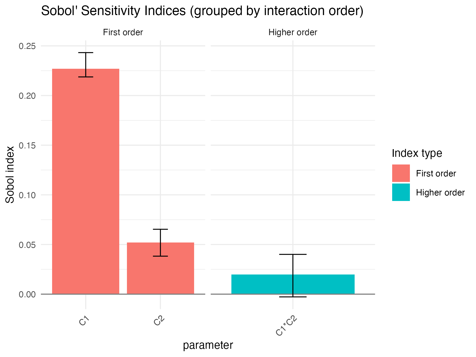

Sobol4R::autoplot(x4)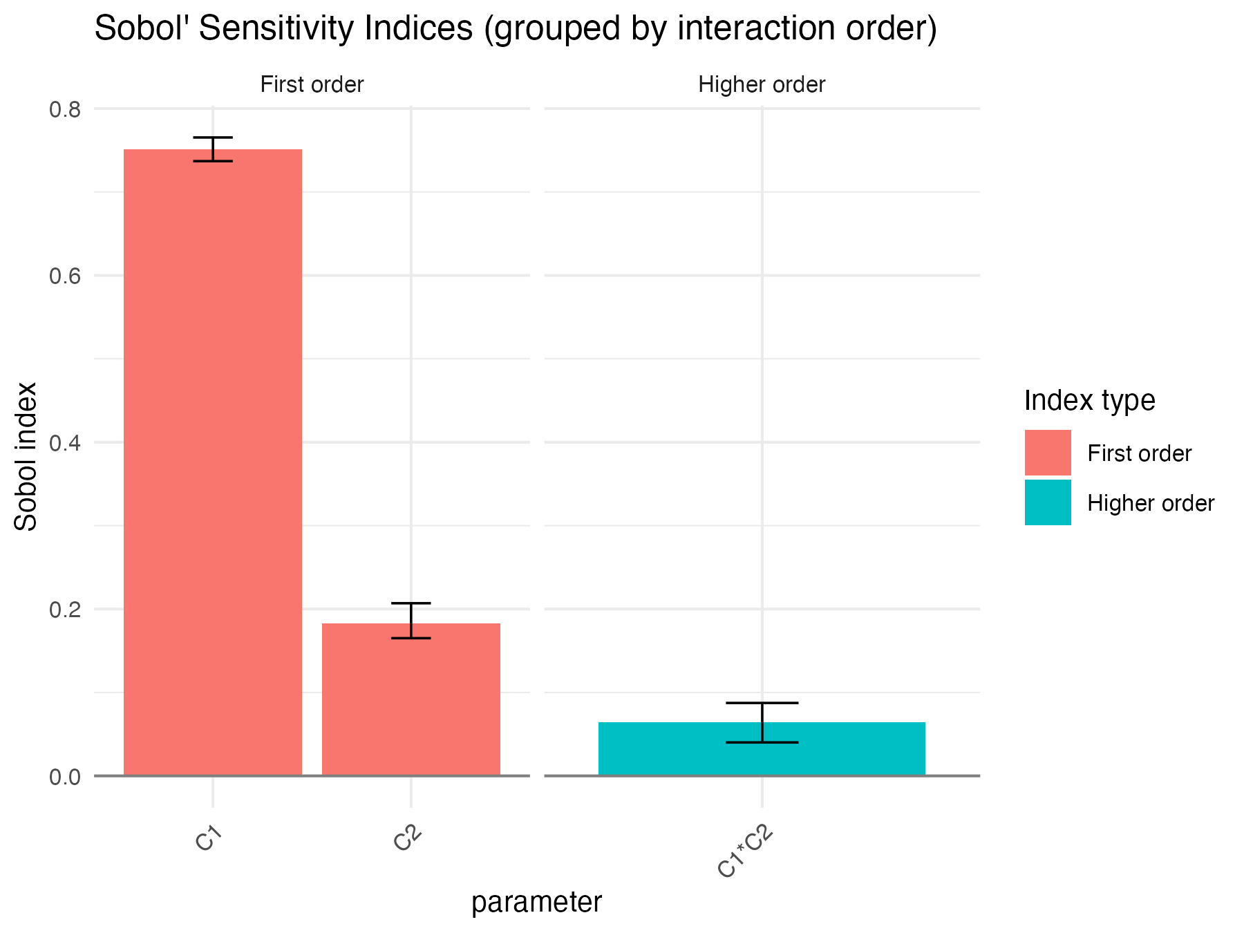

ex2_results <- sobol_example_random_output()
ex2_results
#> $x_det
#> 
#> Call:
#> sensitivity::sobol(model = NULL, X1 = X1, X2 = X2, order = order,     nboot = nboot)
#> 
#> Model runs: 200000 
#> 
#> Sobol indices
#>         original          bias  std. error  min. c.i.  max. c.i.
#> C1    0.74720121 -0.0009978294 0.006004805 0.73615388 0.76091767
#> C2    0.18170442 -0.0018454055 0.010212362 0.16292464 0.20101671
#> C1*C2 0.07113984  0.0028432598 0.013149485 0.04316529 0.09515417
#> 
#> $x_noise
#> 
#> Call:
#> sensitivity::sobol(model = NULL, X1 = X1, X2 = X2, order = order,     nboot = nboot)
#> 
#> Model runs: 200000 
#> 
#> Sobol indices
#>         original          bias  std. error   min. c.i.  max. c.i.
#> C1    0.22767375 -0.0007876749 0.006188751 0.215410324 0.24349360
#> C2    0.05176659  0.0002594516 0.006870501 0.037425458 0.06510662
#> C1*C2 0.02423485 -0.0004615309 0.010009320 0.005753248 0.04323218
#> 
#> $x_qoi
#> 
#> Call:
#> sensitivity::sobol(model = NULL, X1 = X1, X2 = X2, order = order,     nboot = nboot)
#> 
#> Model runs: 200000 
#> 
#> Sobol indices
#>         original          bias  std. error  min. c.i.  max. c.i.
#> C1    0.74586708 -0.0008082631 0.006456912 0.73317476 0.76085938
#> C2    0.18166520 -0.0004252401 0.008343277 0.16630470 0.19952893
#> C1*C2 0.07020214  0.0012650855 0.010728603 0.04892424 0.09107463

Sobol4R::autoplot(ex2_results$x_det)

Sobol4R::autoplot(ex2_results$x_noise)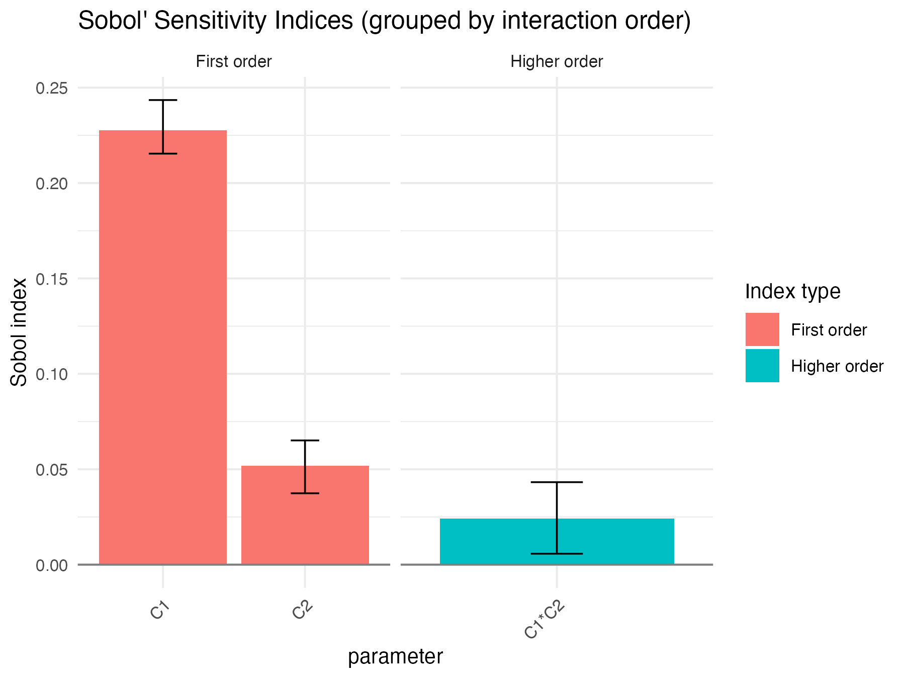

Sobol4R::autoplot(ex2_results$x_qoi)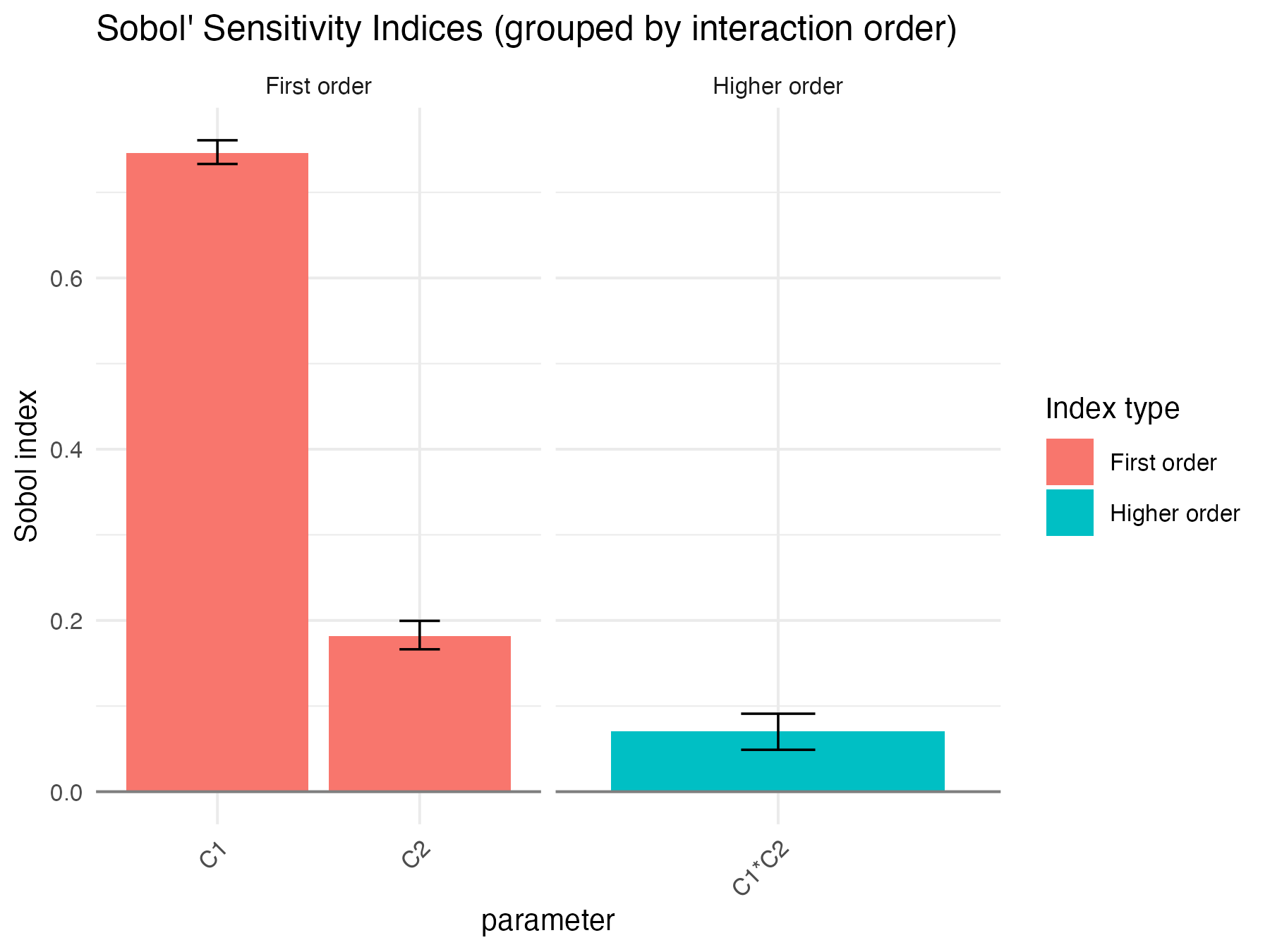

rm(ex2_results)

Sobol and randomness II: large random effect depending on an input variable

We keep the previously generated values for C1 and C2 and add a third variable C3 distributed as runif(n, min = 1, max = 100). The third variable controls the mean of the Gaussian noise.

n <- 50000
X1_r2 <- data.frame(
  C1 = X1_r1$C1,
  C2 = X1_r1$C2,
  C3 = runif(n, min = 1, max = 100)
)
X2_r2 <- data.frame(
  C1 = X2_r1$C1,
  C2 = X2_r1$C2,
  C3 = runif(n, min = 1, max = 100)
)

head(X1_r1)
#>           C1        C2
#> 1 0.01651413 0.8730539
#> 2 0.41411830 0.9350212
#> 3 0.56474556 0.2305029
#> 4 0.19459702 0.5419644
#> 5 0.14134094 0.7620684
#> 6 0.80140480 0.7306451
head(X1_r2)
#>           C1        C2        C3
#> 1 0.01651413 0.8730539 91.158310
#> 2 0.41411830 0.9350212 94.475260
#> 3 0.56474556 0.2305029 18.569825
#> 4 0.19459702 0.5419644 27.675334
#> 5 0.14134094 0.7620684 95.994602
#> 6 0.80140480 0.7306451  6.472291

set.seed(4669)
gensol3 <- sobol4r_design(
  X1    = X1_r2,
  X2    = X2_r2,
  order = 2,
  nboot = 100
)

Y5 <- sobol_g2_with_covariate_noise(gensol3$X)
Y6 <- sobol_g2_qoi_covariate_mean(gensol3$X, nrep = 1000)

x5 <- sensitivity::tell(gensol3, Y5)
x6 <- sensitivity::tell(gensol3, Y6)

print(x5)
#> 
#> Call:
#> sensitivity::sobol(model = NULL, X1 = X1, X2 = X2, order = order,     nboot = nboot)
#> 
#> Model runs: 350000 
#> 
#> Sobol indices
#>           original          bias   std. error   min. c.i.  max. c.i.
#> C1     0.009103922 -7.678676e-04 0.0130427012 -0.01411765 0.03609438
#> C2     0.008522672 -8.213264e-04 0.0131436196 -0.01523813 0.03560910
#> C3     0.997881023  1.842165e-05 0.0005691673  0.99664601 0.99899637
#> C1*C2 -0.008632762  7.862693e-04 0.0130956857 -0.03574270 0.01484363
#> C1*C3 -0.008739565  7.650162e-04 0.0130892998 -0.03539612 0.01503036
#> C2*C3 -0.009249140  7.983501e-04 0.0131952308 -0.03644359 0.01477755
print(x6)
#> 
#> Call:
#> sensitivity::sobol(model = NULL, X1 = X1, X2 = X2, order = order,     nboot = nboot)
#> 
#> Model runs: 350000 
#> 
#> Sobol indices
#>           original          bias   std. error   min. c.i.  max. c.i.
#> C1     0.009294127 -1.646939e-03 0.0119136613 -0.01048769 0.03632675
#> C2     0.008880986 -1.660606e-03 0.0119297217 -0.01065891 0.03604884
#> C3     0.999598476 -5.438879e-05 0.0002670567  0.99915305 1.00020923
#> C1*C2 -0.008767366  1.686318e-03 0.0119169108 -0.03594583 0.01083755
#> C1*C3 -0.008944792  1.678635e-03 0.0119154037 -0.03613794 0.01063203
#> C2*C3 -0.008945624  1.673590e-03 0.0119138645 -0.03611414 0.01064228

Sobol4R::autoplot(x5)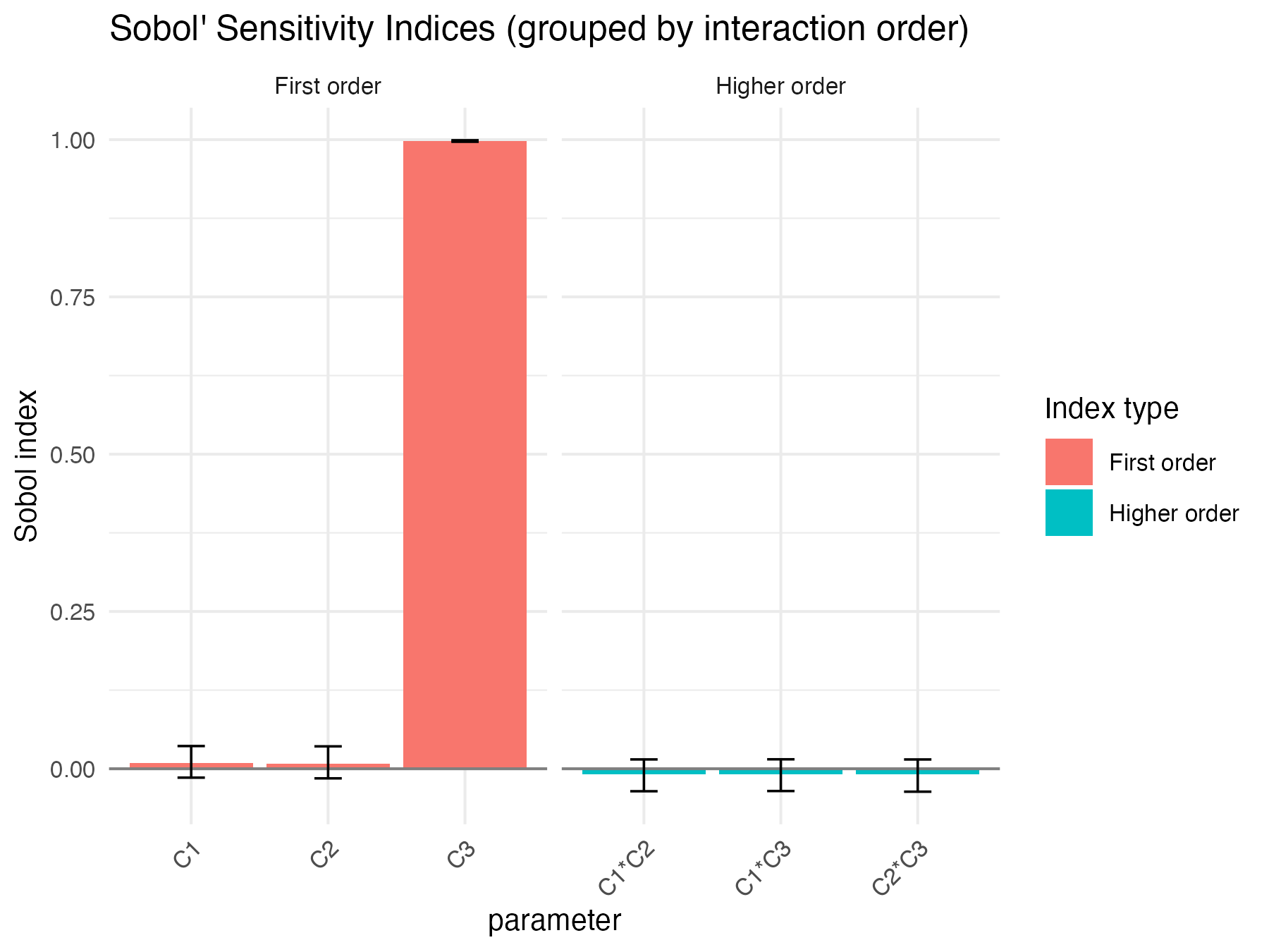

Sobol4R::autoplot(x6)

ex3_results <- sobol_example_covariate_large()
ex3_results
#> $x_single
#> 
#> Call:
#> sensitivity::sobol(model = NULL, X1 = X1, X2 = X2, order = order,     nboot = nboot)
#> 
#> Model runs: 350000 
#> 
#> Sobol indices
#>           original          bias   std. error   min. c.i.  max. c.i.
#> C1    -0.003814153  2.616697e-03 0.0125631569 -0.02644550 0.02762452
#> C2    -0.003825927  2.659501e-03 0.0125560080 -0.02648521 0.02766639
#> C3     0.997455455 -7.568744e-06 0.0005209994  0.99636991 0.99856976
#> C1*C2  0.003820640 -2.669221e-03 0.0125262397 -0.02766157 0.02691652
#> C1*C3  0.004519403 -2.631650e-03 0.0125653953 -0.02710749 0.02681053
#> C2*C3  0.004166187 -2.636226e-03 0.0126073022 -0.02770878 0.02685501
#> 
#> $x_qoi
#> 
#> Call:
#> sensitivity::sobol(model = NULL, X1 = X1, X2 = X2, order = order,     nboot = nboot)
#> 
#> Model runs: 350000 
#> 
#> Sobol indices
#>           original          bias   std. error   min. c.i.  max. c.i.
#> C1    -0.003563336  5.722503e-04 0.0113799469 -0.02940469 0.01662036
#> C2    -0.004120807  5.684572e-04 0.0114033647 -0.02959945 0.01580905
#> C3     0.999489107  1.507974e-05 0.0003031387  0.99874021 1.00009533
#> C1*C2  0.004119381 -5.850545e-04 0.0113790237 -0.01582253 0.02971439
#> C1*C3  0.004146628 -5.696827e-04 0.0113793001 -0.01588901 0.02971427
#> C2*C3  0.004119570 -5.706827e-04 0.0113799985 -0.01592504 0.02970237

Sobol4R::autoplot(ex3_results$x_single)

Sobol4R::autoplot(ex3_results$x_qoi)

rm(ex3_results)

Sobol and randomness III: slight random effect depending on an input variable

We now take a third input C3 distributed as runif(n, min = 1, max = 1.5), which induces a much smaller range for the mean of the noise.

n <- 50000
X1_r3 <- data.frame(
  C1 = X1_r1$C1,
  C2 = X1_r1$C2,
  C3 = runif(n, min = 1, max = 1.5)
)
X2_r3 <- data.frame(
  C1 = X2_r1$C1,
  C2 = X2_r1$C2,
  C3 = runif(n, min = 1, max = 1.5)
)

set.seed(4669)
gensol4 <- sobol4r_design(
  X1    = X1_r3,
  X2    = X2_r3,
  order = 2,
  nboot = 100
)

Y7 <- sobol_g2_with_covariate_noise(gensol4$X)
Y8 <- sobol_g2_qoi_covariate_mean(gensol4$X, nrep = 1000)

x7 <- sensitivity::tell(gensol4, Y7)
x8 <- sensitivity::tell(gensol4, Y8)

print(x7)
#> 
#> Call:
#> sensitivity::sobol(model = NULL, X1 = X1, X2 = X2, order = order,     nboot = nboot)
#> 
#> Model runs: 350000 
#> 
#> Sobol indices
#>            original          bias std. error    min. c.i.  max. c.i.
#> C1     0.2179768074  0.0016590219 0.01191680  0.191936435 0.23884604
#> C2     0.0438787602  0.0002946957 0.01299949  0.014190486 0.06778009
#> C3     0.0012709850  0.0009372044 0.01300281 -0.027475579 0.02831144
#> C1*C2  0.0291744931 -0.0003934838 0.01952600 -0.002590527 0.07333499
#> C1*C3  0.0048315721 -0.0017972989 0.01764631 -0.029694591 0.04260449
#> C2*C3 -0.0001193627 -0.0013974652 0.01639057 -0.030860059 0.04118317
print(x8)
#> 
#> Call:
#> sensitivity::sobol(model = NULL, X1 = X1, X2 = X2, order = order,     nboot = nboot)
#> 
#> Model runs: 350000 
#> 
#> Sobol indices
#>           original         bias std. error    min. c.i.  max. c.i.
#> C1     0.722991696 -0.002288327 0.01354553  0.699849145 0.75130274
#> C2     0.172823871 -0.003699652 0.01778973  0.130371959 0.21764120
#> C3     0.051463767 -0.003001862 0.01984986  0.011515221 0.09988415
#> C1*C2  0.060605565  0.004948431 0.02333160  0.006445535 0.10587228
#> C1*C3 -0.009441546  0.004124036 0.02096216 -0.060569278 0.03514172
#> C2*C3 -0.009732205  0.004024467 0.02083542 -0.060257137 0.03574496

Sobol4R::autoplot(x7)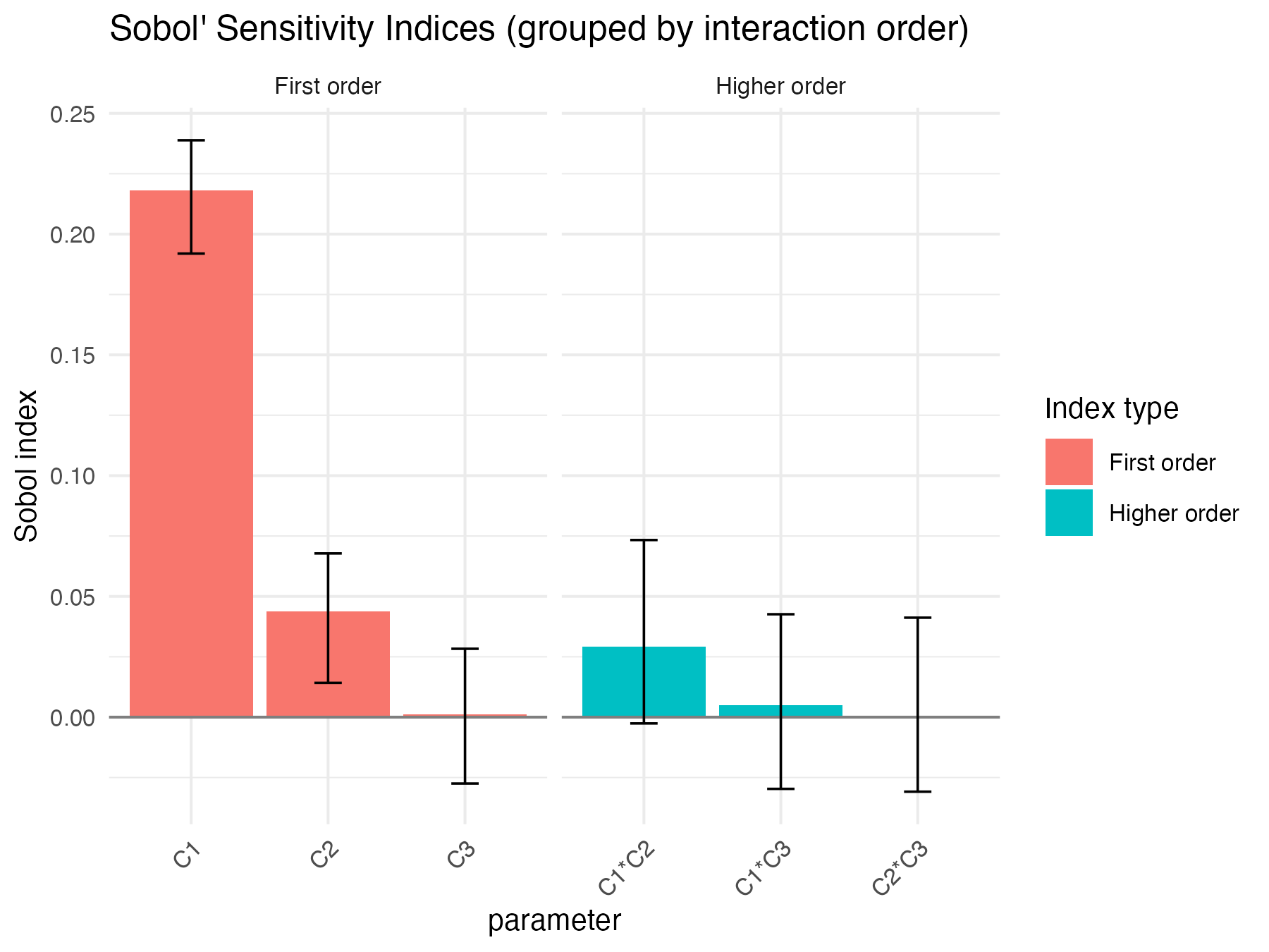

Sobol4R::autoplot(x8)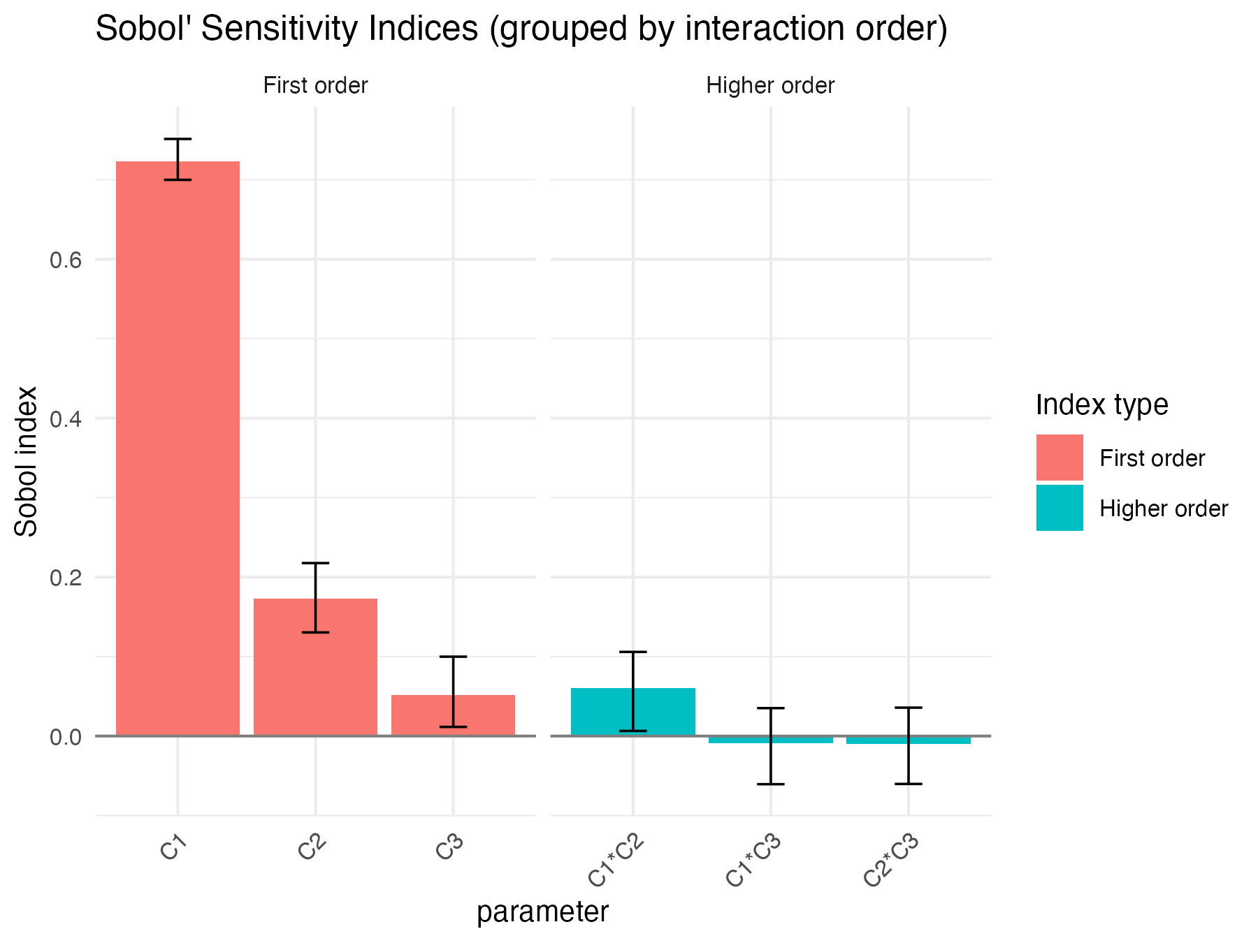

ex4_results <- sobol_example_covariate_small()
ex4_results
#> $x_single
#> 
#> Call:
#> sensitivity::sobol(model = NULL, X1 = X1, X2 = X2, order = order,     nboot = nboot)
#> 
#> Model runs: 350000 
#> 
#> Sobol indices
#>           original          bias std. error   min. c.i.  max. c.i.
#> C1     0.224208081  0.0012907769 0.01092529  0.20087926 0.24485842
#> C2     0.047462732  0.0020584734 0.01175320  0.02042534 0.06960328
#> C3    -0.002896607 -0.0007483782 0.01198692 -0.02880861 0.02251407
#> C1*C2  0.013175351 -0.0025822109 0.01817007 -0.01795887 0.05058618
#> C1*C3  0.004942585 -0.0008555590 0.01442329 -0.02767290 0.03497922
#> C2*C3  0.013227984 -0.0021602752 0.01718477 -0.02285421 0.05404896
#> 
#> $x_qoi
#> 
#> Call:
#> sensitivity::sobol(model = NULL, X1 = X1, X2 = X2, order = order,     nboot = nboot)
#> 
#> Model runs: 350000 
#> 
#> Sobol indices
#>          original         bias std. error    min. c.i.  max. c.i.
#> C1     0.72703512  0.001086299 0.01254459  0.696919113 0.74615423
#> C2     0.17877081  0.002398711 0.02056101  0.137445422 0.22378421
#> C3     0.06021278  0.002800955 0.02095518  0.010950727 0.10250190
#> C1*C2  0.04336379 -0.003300194 0.02578821 -0.006492632 0.10452521
#> C1*C3 -0.01158259 -0.002973672 0.02095654 -0.056111648 0.03698519
#> C2*C3 -0.01328830 -0.003029785 0.02103294 -0.056820767 0.03617793

Sobol4R::autoplot(ex4_results$x_single)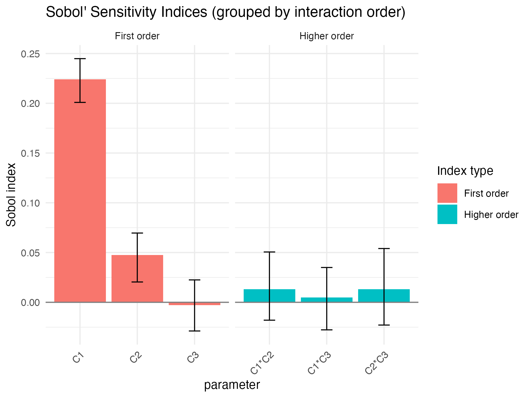

Sobol4R::autoplot(ex4_results$x_qoi)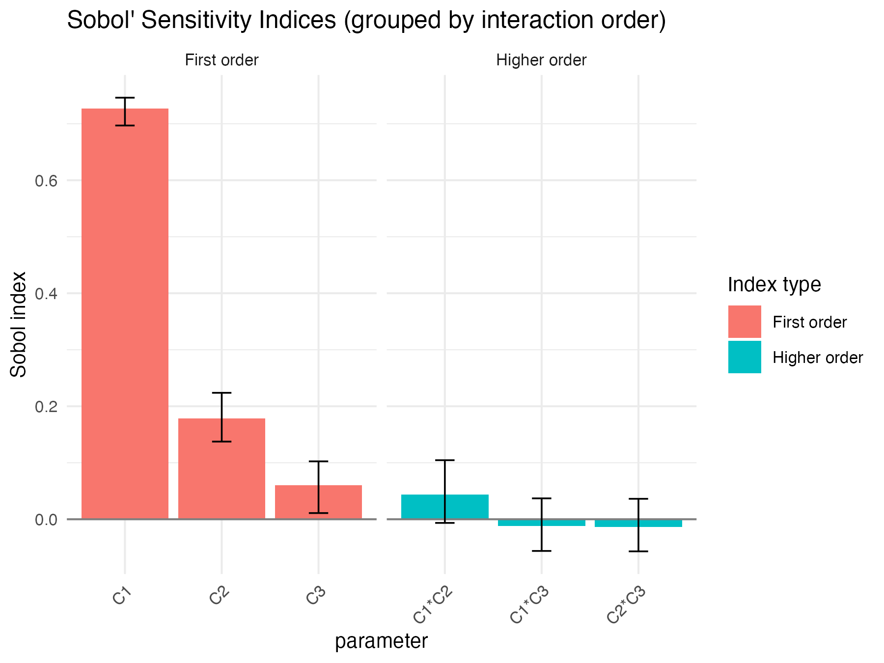

rm(ex4_results)

Sobol and randomness IV: random variables with fixed distribution parameters

We now turn to the process model. The uncertain inputs are the distributional parameters of the individual unit model. The quantity of interest is the time needed to reach a given number of successes.

n <- 100

draw_params <- function(n) {
  data.frame(t(replicate(
    n,
    c(
      1 / runif(1, min = 20,  max = 100),
      1 / runif(1, min = 24,  max = 2000),
      1 / runif(1, min = 24,  max = 120),
      runif(1,  min = 0.05, max = 0.3),
      runif(1,  min = 0.3,  max = 0.7)
    )
  )))
}

X1_process <- draw_params(n)
X2_process <- draw_params(n)

set.seed(4669)
gensolp1 <- sobol4r_design(
  X1    = X1_process,
  X2    = X2_process,
  order = 2,
  nboot = 10
)

MM <- 50

Yp1 <- process_fun_row_wise(gensolp1$X, M = MM)
Yp2 <- process_fun_mean_to_M(gensolp1$X, M = MM, nrep = 10)

xp1 <- sensitivity::tell(gensolp1, Yp1)
xp2 <- sensitivity::tell(gensolp1, Yp2)

print(xp1)
#> 
#> Call:
#> sensitivity::sobol(model = NULL, X1 = X1, X2 = X2, order = order,     nboot = nboot)
#> 
#> Model runs: 1600 
#> 
#> Sobol indices
#>           original        bias std. error    min. c.i. max. c.i.
#> X1     0.380640729  0.07767979  0.1894920 -0.097930324 0.5209198
#> X2    -0.150879591  0.04386871  0.1879200 -0.465393405 0.1238071
#> X3    -0.184757024  0.04843735  0.1744516 -0.521524088 0.0152424
#> X4     0.116097870  0.09833723  0.3563339 -0.528448252 0.7365426
#> X5     0.008791147  0.06817654  0.1774518 -0.295431490 0.1728399
#> X1*X2  0.158754474 -0.08122172  0.1639657  0.003120269 0.4764820
#> X1*X3  0.132555870 -0.04669304  0.1412632 -0.011660608 0.4174054
#> X1*X4  0.265193836 -0.18009652  0.2617729  0.116915514 0.9749080
#> X1*X5  0.265493347 -0.12287799  0.2249038  0.092587933 0.6875449
#> X2*X3  0.181003438 -0.02326317  0.1711716 -0.030749675 0.4964048
#> X2*X4  0.164670426 -0.07306096  0.2230941 -0.109832214 0.5971065
#> X2*X5  0.185335203 -0.05811882  0.1953846 -0.060305511 0.5041611
#> X3*X4  0.166022145 -0.12110900  0.2730700 -0.069392144 0.8097652
#> X3*X5  0.145940968 -0.02318531  0.1665974 -0.036930422 0.4135084
#> X4*X5  0.075804433 -0.12414127  0.2503957 -0.175048932 0.6206474
print(xp2)
#> 
#> Call:
#> sensitivity::sobol(model = NULL, X1 = X1, X2 = X2, order = order,     nboot = nboot)
#> 
#> Model runs: 1600 
#> 
#> Sobol indices
#>          original         bias std. error    min. c.i.   max. c.i.
#> X1     0.28552380 -0.004625494  0.1629528 -0.025026380  0.55227506
#> X2    -0.24716893  0.040791568  0.1852317 -0.620146362 -0.03364271
#> X3    -0.26283415  0.037441973  0.1828269 -0.624282749 -0.04747583
#> X4    -0.01106905  0.096595668  0.2098145 -0.650270117  0.11074470
#> X5    -0.06103096  0.010017363  0.1833158 -0.485658110  0.18766248
#> X1*X2  0.25974232 -0.042769338  0.1837775  0.050259571  0.61829376
#> X1*X3  0.24974787 -0.031849303  0.1708788  0.030397575  0.56635633
#> X1*X4  0.41897897 -0.053364983  0.2031692  0.118286391  0.79615594
#> X1*X5  0.30368407 -0.042679127  0.1907361  0.106453978  0.67277643
#> X2*X3  0.25732160 -0.045545310  0.1922518  0.033573909  0.63719282
#> X2*X4  0.25958598 -0.036109212  0.1916288  0.043772771  0.64322604
#> X2*X5  0.23572522 -0.038548190  0.1814357  0.032204334  0.58719703
#> X3*X4  0.26487283 -0.035018351  0.1725196  0.057452499  0.59887908
#> X3*X5  0.23794077 -0.038174061  0.1819509  0.024176202  0.61056056
#> X4*X5  0.28769557 -0.010575839  0.1950144  0.007294713  0.67587200

Sobol4R::autoplot(xp1)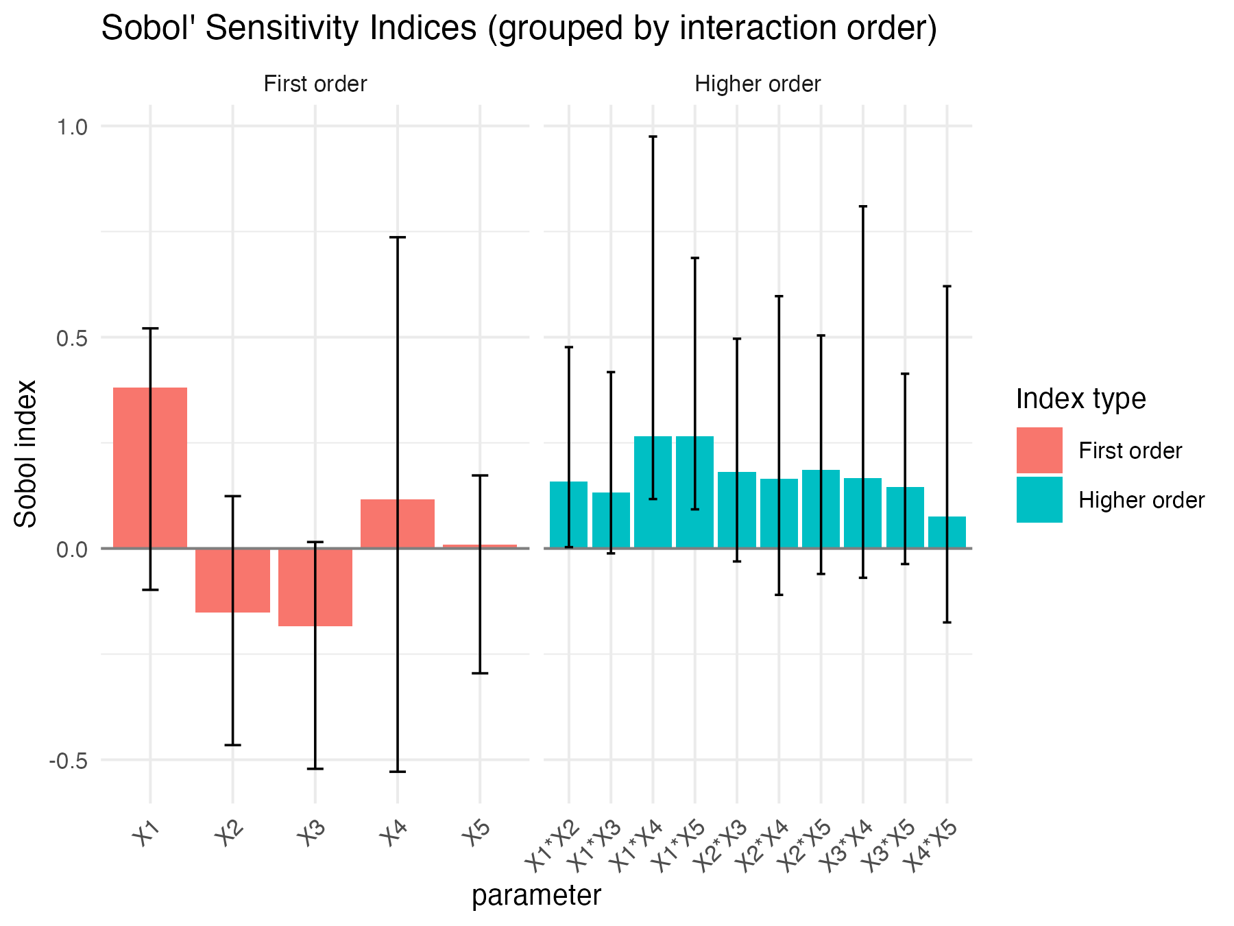

Sobol4R::autoplot(xp2)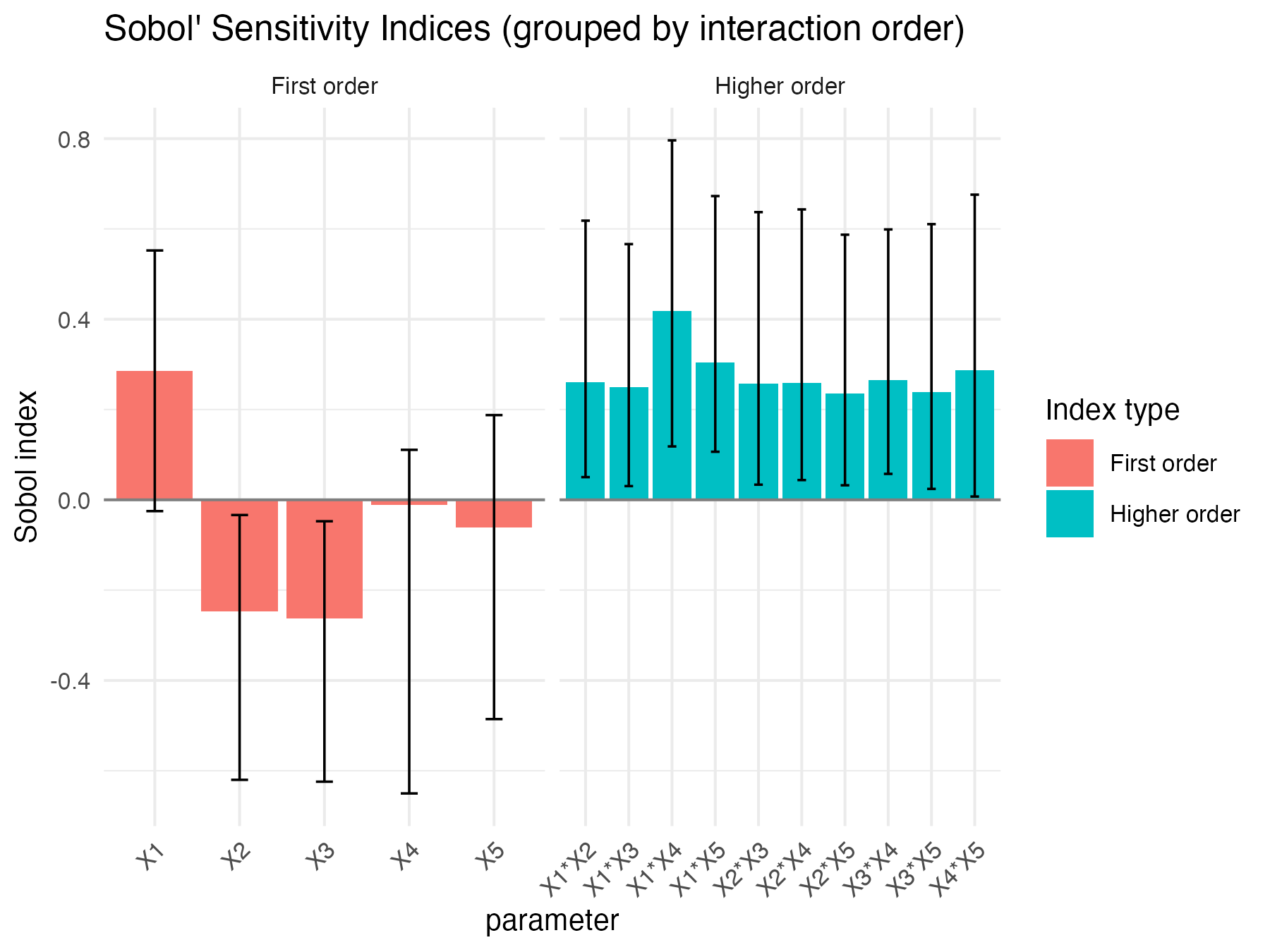

ex5_results <- sobol_example_process(order = 2)
ex5_results
#> $xp_single
#> 
#> Call:
#> sensitivity::sobol(model = NULL, X1 = X1, X2 = X2, order = order,     nboot = nboot)
#> 
#> Model runs: 1600 
#> 
#> Sobol indices
#>          original         bias std. error   min. c.i. max. c.i.
#> X1     0.46181191  0.038167121  0.1015640  0.33795565 0.6441305
#> X2    -0.13443272  0.037980913  0.2138908 -0.40535715 0.2940413
#> X3    -0.18784544  0.023277680  0.2225694 -0.36793913 0.3174555
#> X4     0.21539857  0.072332580  0.2527034 -0.15248847 0.6363769
#> X5    -0.08619123  0.023396235  0.2452619 -0.46074941 0.3720733
#> X1*X2  0.02965770 -0.054444661  0.2173068 -0.39209351 0.3442244
#> X1*X3  0.08115352 -0.026507036  0.2471829 -0.44675755 0.2948945
#> X1*X4  0.25096547 -0.023941343  0.3122315 -0.29482004 0.5329074
#> X1*X5  0.07311200 -0.120037030  0.3016293 -0.32207953 0.7162746
#> X2*X3  0.29404175 -0.008448518  0.1835533 -0.10975779 0.5326415
#> X2*X4  0.19699573 -0.039574605  0.2031531 -0.23590639 0.4058620
#> X2*X5  0.10531152 -0.041042052  0.2247256 -0.34402148 0.4190775
#> X3*X4  0.26918894 -0.040096061  0.1790315 -0.06567867 0.5182382
#> X3*X5  0.16210360 -0.015655387  0.2790156 -0.51100724 0.4133400
#> X4*X5  0.38191573 -0.050617095  0.2409964 -0.06624024 0.8481388
#> 
#> $xp_qoi
#> 
#> Call:
#> sensitivity::sobol(model = NULL, X1 = X1, X2 = X2, order = order,     nboot = nboot)
#> 
#> Model runs: 1600 
#> 
#> Sobol indices
#>          original         bias std. error   min. c.i. max. c.i.
#> X1     0.43347914 -0.045976744  0.1845412  0.03886395 0.6400869
#> X2    -0.13026450  0.025599145  0.1872325 -0.34701259 0.1252922
#> X3    -0.11367591  0.021728558  0.1872673 -0.34349970 0.1328036
#> X4     0.32339355  0.031687132  0.1869744  0.01019336 0.5028818
#> X5    -0.03466342  0.012537251  0.2486094 -0.36356182 0.2985800
#> X1*X2  0.16423345 -0.035038812  0.2134525 -0.13986660 0.4309059
#> X1*X3  0.09499188 -0.013329557  0.1932010 -0.18465828 0.3481033
#> X1*X4  0.25284389  0.026563603  0.2528613 -0.21294867 0.5635387
#> X1*X5  0.08488172 -0.036702375  0.2161232 -0.16361182 0.4289381
#> X2*X3  0.09966690 -0.021597414  0.1964646 -0.16909004 0.3289556
#> X2*X4  0.14229878 -0.026644351  0.1867969 -0.12375633 0.3585671
#> X2*X5  0.13160860 -0.009979547  0.1886424 -0.12347665 0.3548174
#> X3*X4  0.10512121 -0.022765838  0.1848153 -0.13590512 0.3306203
#> X3*X5  0.09985455 -0.009063853  0.1981656 -0.15621906 0.3938962
#> X4*X5  0.16815214 -0.045139164  0.1669667 -0.03943283 0.4053975

Sobol4R::autoplot(ex5_results$xp_single)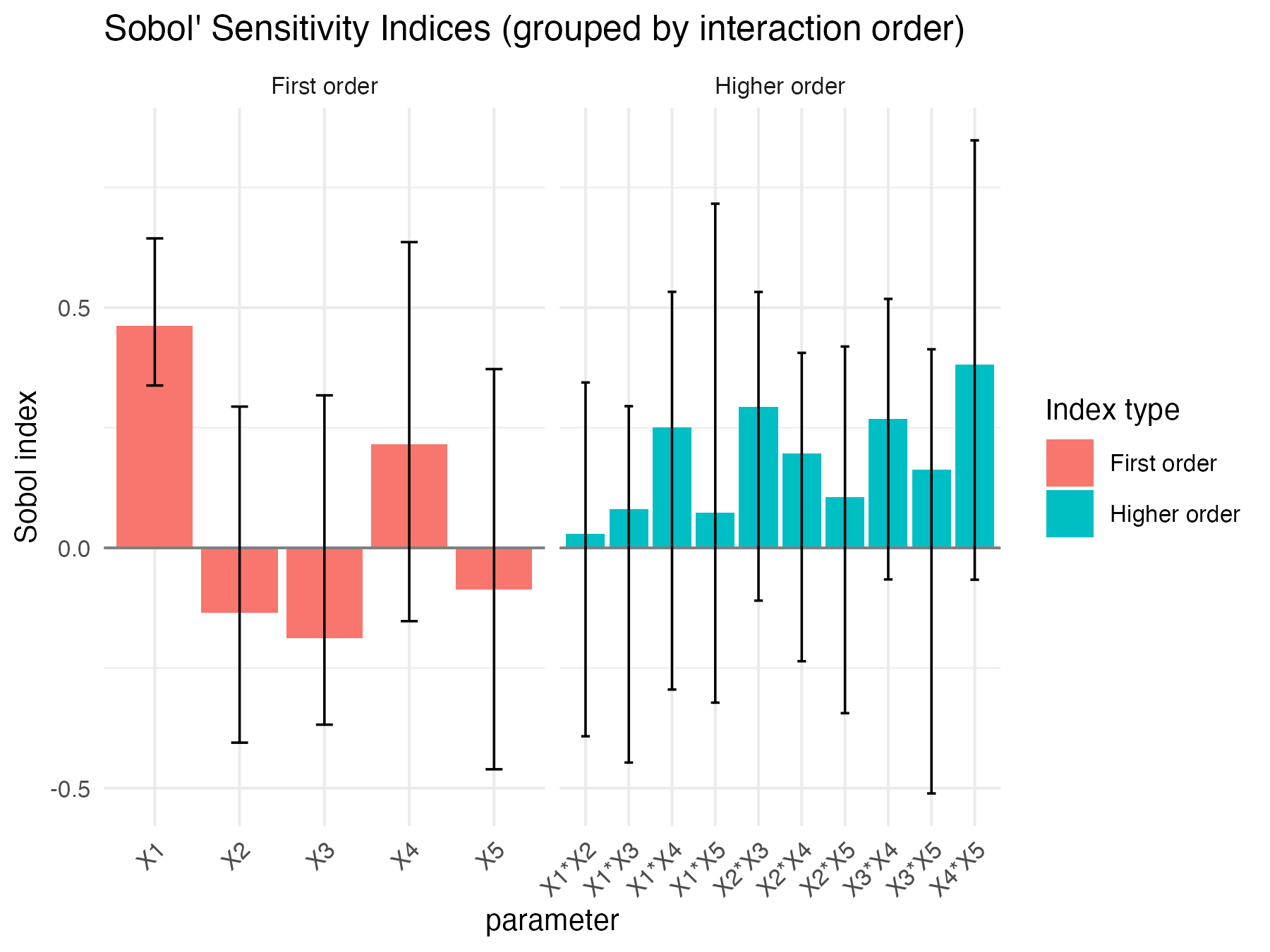

Sobol4R::autoplot(ex5_results$xp_qoi)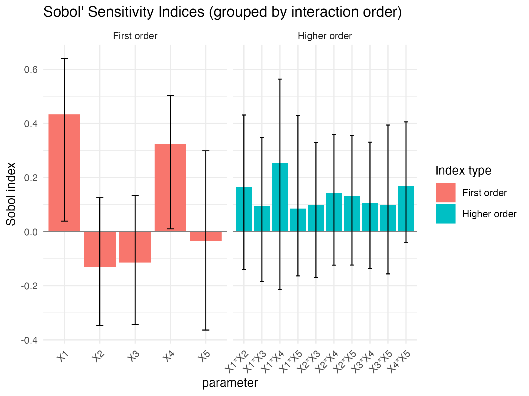

rm(ex5_results)

Frédéric Bertrand