Sobol4R: Sobol indices for stochastic models
Frédéric Bertrand
Cedric, Cnam, Parisfrederic.bertrand@lecnam.net
2025-11-27
Source:vignettes/Sobol4R_vignette_stochastic.Rmd
Sobol4R_vignette_stochastic.RmdIntroduction
This vignette illustrates the use of the Sobol4R package to compute Sobol indices for deterministic and stochastic versions of the classical Sobol g function.
The designs are generated with sensitivity::sobol and
the models are provided by Sobol4R, in particular
-
sobol_g_functionfor the deterministic g function
-
sobol_g2_additive_noisefor a version of the model with additive Gaussian noise
-
sobol_g2_with_covariate_noisefor a version with covariate dependent noise
The stochastic models can be combined with the generic quantity of
interest wrapper sobol4r_qoi.
Deterministic Sobol g function
Order 1 and Total via sensitivity::sobol()
n  <- 1e4
p  <- 8
X1 <- data.frame(matrix(runif(p * n), nrow = n))
X2 <- data.frame(matrix(runif(p * n), nrow = n))

sob_det <- sobol4r_design(X1 = X1, X2 = X2, order = 2, nboot = 50)

Y <- sobol_g_function(sob_det$X)
sensitivity::tell(sob_det, Y)
print(sob_det)
#>
#> Call:
#> sensitivity::soboljansen(model = NULL, X1 = X1, X2 = X2, nboot = nboot)
#>
#> Model runs: 100000
#>
#> First order indices:
#>       original          bias  std. error    min. c.i.  max. c.i.
#> X1 0.717660678 -0.0009932676 0.006036444  0.704737206 0.73253886
#> X2 0.185342302 -0.0020706753 0.014354599  0.154165726 0.21333266
#> X3 0.024134416 -0.0025884308 0.014211364 -0.007872698 0.05741629
#> X4 0.013559153 -0.0038402521 0.014099271 -0.016977087 0.04874150
#> X5 0.005864082 -0.0037560690 0.014028598 -0.022414985 0.04106775
#> X6 0.005796217 -0.0038042037 0.014036002 -0.022355436 0.04105654
#> X7 0.005778092 -0.0037573736 0.013989862 -0.022549033 0.04100004
#> X8 0.006151195 -0.0036990459 0.014049146 -0.021865015 0.04120230
#>
#> Total indices:
#>        original          bias   std. error    min. c.i.    max. c.i.
#> X1 0.7684270334  1.348517e-03 1.095303e-02 7.451818e-01 0.7922941591
#> X2 0.2391940077  2.015426e-04 4.097996e-03 2.302565e-01 0.2478394129
#> X3 0.0333164459  6.195538e-05 6.267740e-04 3.199008e-02 0.0346766967
#> X4 0.0104979835  2.557619e-05 2.824431e-04 9.884158e-03 0.0109966841
#> X5 0.0001033816  1.375728e-09 1.732832e-06 1.000611e-04 0.0001068481
#> X6 0.0001053492 -1.117878e-07 2.656393e-06 9.829080e-05 0.0001102474
#> X7 0.0001039507  7.510483e-08 2.285392e-06 9.790305e-05 0.0001085273
#> X8 0.0001006685  2.460455e-07 2.009040e-06 9.605339e-05 0.0001040869
Sobol4R::autoplot(sob_det, ncol = 1)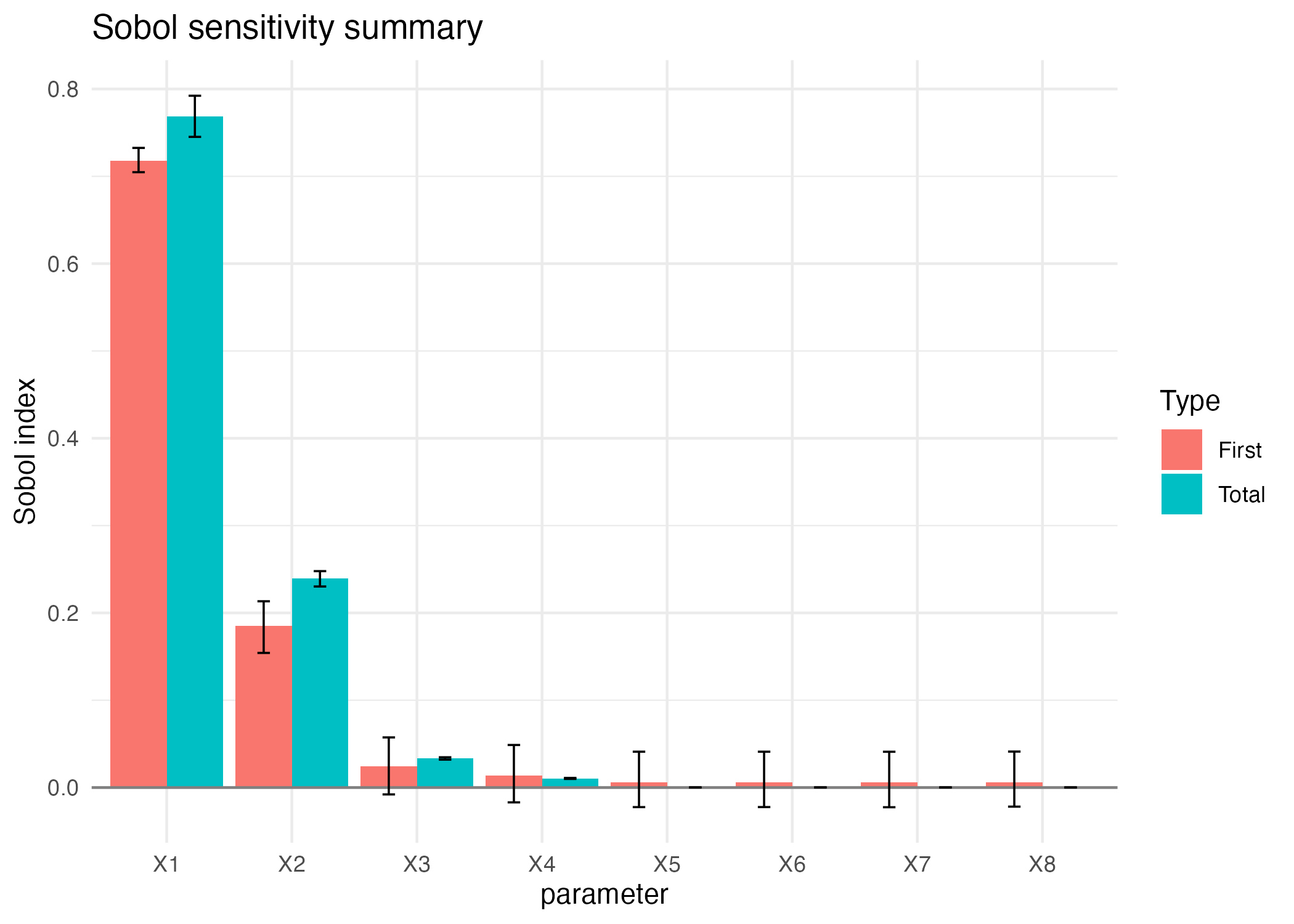
Order 1 and Total via sensitivity::sobol2007()
n  <- 1e4
p  <- 8
X1 <- data.frame(matrix(runif(p * n), nrow = n))
X2 <- data.frame(matrix(runif(p * n), nrow = n))

sob_det_2007 <- sobol4r_design(
  X1    = X1,
  X2    = X2,
  nboot = 50,
  type  = "sobol2007"
)

Y <- sobol_g_function(sob_det_2007$X)
sensitivity::tell(sob_det_2007, Y)
print(sob_det_2007)
#>
#> Call:
#> sensitivity::sobol2007(model = NULL, X1 = X1, X2 = X2, nboot = nboot)
#>
#> Model runs: 100000
#>
#> First order indices:
#>         original          bias   std. error     min. c.i.    max. c.i.
#> X1  7.226361e-01  4.613664e-04 0.0250889263  0.6714746826 0.7732251982
#> X2  1.577506e-01  1.759382e-03 0.0147669207  0.1267157769 0.1960646433
#> X3  2.165769e-02 -1.967632e-04 0.0048301391  0.0107498709 0.0330404949
#> X4  6.966461e-03  2.491303e-04 0.0027234991  0.0010555430 0.0110881879
#> X5  2.104365e-04  5.952562e-05 0.0002402671 -0.0003020478 0.0005739324
#> X6  2.982284e-04  6.010743e-05 0.0002228694 -0.0003302314 0.0007606267
#> X7  5.419411e-05 -3.806394e-05 0.0001951958 -0.0002465745 0.0005861267
#> X8 -1.885046e-04  4.378118e-05 0.0002970498 -0.0009607355 0.0003931021
#>
#> Total indices:
#>         original          bias   std. error     min. c.i.    max. c.i.
#> X1  0.8114688026  1.482182e-03 0.0209887057  0.7632449114 0.8584297401
#> X2  0.2657395655  9.298296e-04 0.0162802955  0.2268143380 0.3035468573
#> X3  0.0380832600  7.402175e-04 0.0070172023  0.0199547275 0.0506997801
#> X4  0.0080414206 -4.546740e-04 0.0040901847 -0.0006915014 0.0172996762
#> X5 -0.0000740697 -9.898440e-05 0.0004524606 -0.0010437911 0.0009069280
#> X6  0.0001245399 -8.659793e-05 0.0003678083 -0.0006133636 0.0011593635
#> X7  0.0001987163  2.279008e-05 0.0003327657 -0.0004079122 0.0007984449
#> X8  0.0007342818 -7.943007e-05 0.0004619398 -0.0003188098 0.0019252166
Sobol4R::autoplot(sob_det_2007)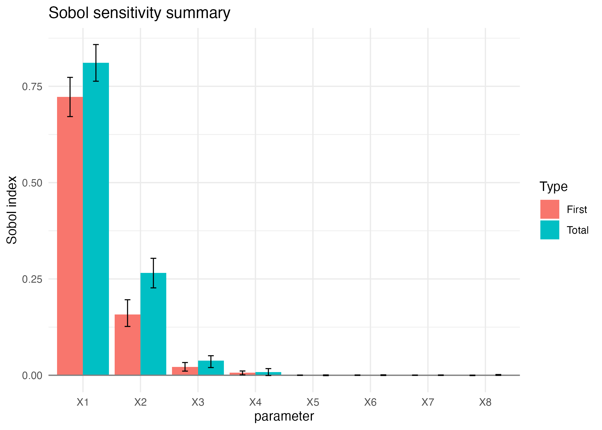
Random effect on the output
We restrict the g function to the first two inputs and add a Gaussian noise term with zero mean and unit variance.
Order 1 and Total via sensitivity::sobol()
sob_noise_add <- sobol4r_design(X1 = X1[, 1:2], X2 = X2[, 1:2], order = 2, nboot = 50, type = "sobol")

Y <- sobol_g2_additive_noise(sob_noise_add$X)
sensitivity::tell(sob_noise_add, Y)
print(sob_noise_add)
#>
#> Call:
#> sensitivity::sobol(model = NULL, X1 = X1, X2 = X2, order = order,     nboot = nboot)
#>
#> Model runs: 40000
#>
#> Sobol indices
#>          original         bias std. error   min. c.i.  max. c.i.
#> X1    0.210591303  0.002895381 0.01339506  0.17772950 0.23133242
#> X2    0.077394970  0.001182011 0.01465379  0.04788607 0.10591187
#> X1*X2 0.004634588 -0.002890048 0.02552980 -0.05706284 0.06587072
Sobol4R::autoplot(sob_noise_add)
Order 1 and Total via sensitivity::sobol2007()
sob_noise_add <- sobol4r_design(X1 = X1[, 1:2], X2 = X2[, 1:2], nboot = 50, type = "sobol2007")

Y <- sobol_g2_additive_noise(sob_noise_add$X)
sensitivity::tell(sob_noise_add, Y)
print(sob_noise_add)
#>
#> Call:
#> sensitivity::sobol2007(model = NULL, X1 = X1, X2 = X2, nboot = nboot)
#>
#> Model runs: 40000
#>
#> First order indices:
#>      original          bias std. error  min. c.i.  max. c.i.
#> X1 0.22249900 -0.0007019890 0.02086091 0.18921641 0.27421970
#> X2 0.04947403  0.0009910796 0.01799606 0.01167035 0.08611989
#>
#> Total indices:
#>     original          bias std. error min. c.i. max. c.i.
#> X1 0.9545870 -1.644061e-03 0.01536769 0.9247617 0.9938948
#> X2 0.7936756  7.622615e-05 0.01269614 0.7679734 0.8230877
Sobol4R::autoplot(sob_noise_add)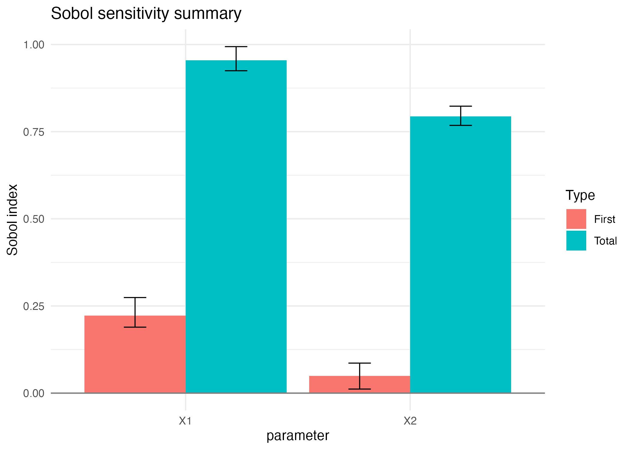
Quantity of interest based on repeated runs
Instead of a single noisy run, we can focus on a quantity of interest, here the conditional mean of the output given the inputs. This is approximated by repeated calls to the stochastic model.
Order 1 and Total via sensitivity::sobol()
sob_noise_const_qoi <- sobol4r_qoi_indices(
  model = sobol_g2_additive_noise,
  X1 = X1[, 1:2],
  X2 = X2[, 1:2],
  order = 2,
  nboot = 50,
  type = "sobol")
print(sob_noise_const_qoi)
#>
#> Call:
#> sensitivity::sobol(model = NULL, X1 = X1, X2 = X2, order = order,     nboot = nboot)
#>
#> Model runs: 40000
#>
#> Sobol indices
#>        original         bias std. error min. c.i. max. c.i.
#> X1    0.7281363 -0.002326129 0.01396703 0.7023478 0.7611659
#> X2    0.1593779  0.001107771 0.02101239 0.1111086 0.1996645
#> X1*X2 0.1115358  0.001362466 0.02579994 0.0601593 0.1660907
Sobol4R::autoplot(sob_noise_const_qoi)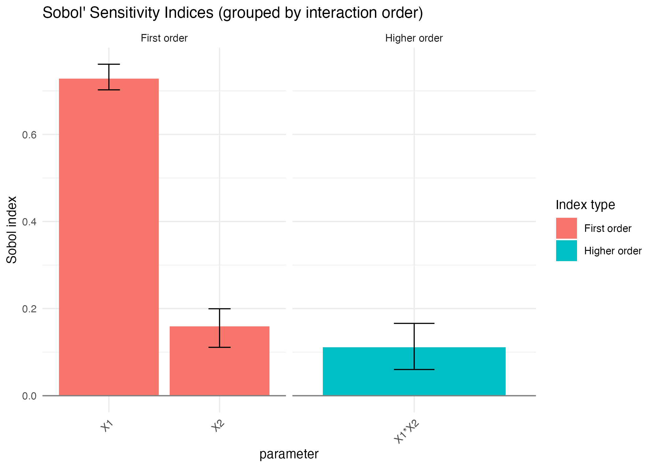
Order 1 and Total via sensitivity::sobol2007()
sob_noise_const_qoi <- sobol4r_qoi_indices(
  model = sobol_g2_additive_noise,
  X1 = X1[, 1:2],
  X2 = X2[, 1:2],
  nboot = 50,
  type = "sobol2007")
print(sob_noise_const_qoi)
#>
#> Call:
#> sensitivity::sobol2007(model = NULL, X1 = X1, X2 = X2, nboot = nboot)
#>
#> Model runs: 40000
#>
#> First order indices:
#>    original         bias  std. error min. c.i. max. c.i.
#> X1 0.778753 0.0041844030 0.013385447 0.7510859 0.8136224
#> X2 0.187627 0.0005980994 0.007046389 0.1712593 0.2009642
#>
#> Total indices:
#>     original         bias  std. error min. c.i. max. c.i.
#> X1 0.8200828  0.002239187 0.009360912 0.7983630 0.8358809
#> X2 0.2540245 -0.001060357 0.006998130 0.2466031 0.2736040
Sobol4R::autoplot(sob_noise_const_qoi)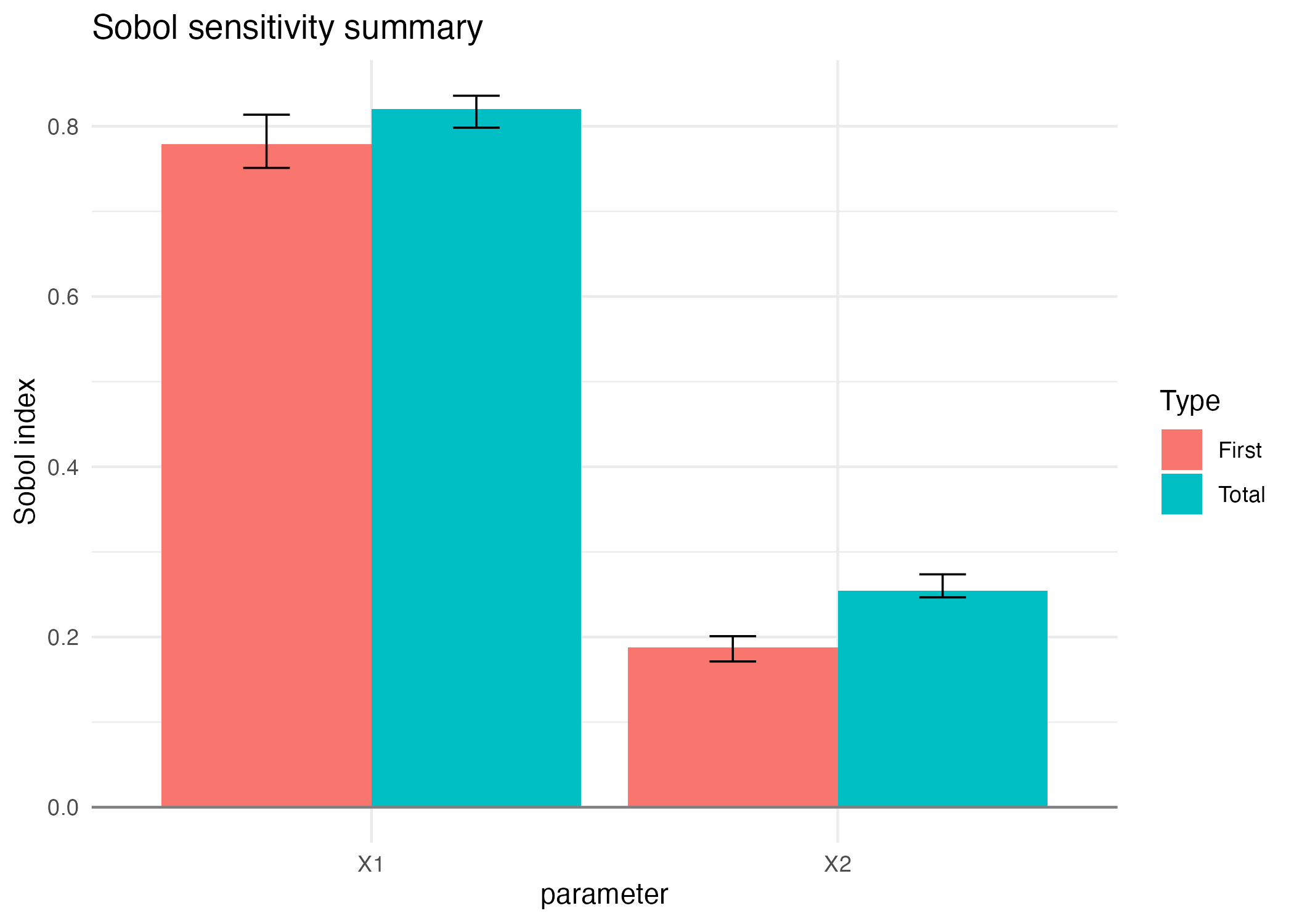
Covariate dependent noise
We now add a third input which controls the mean of the Gaussian noise term. The mean is equal to the third input, and the variance is fixed.
X1_cov <- data.frame(
  C1 = runif(n),
  C2 = runif(n),
  C3 = runif(n, min = 1, max = 100)
)
X2_cov <- data.frame(
  C1 = runif(n),
  C2 = runif(n),
  C3 = runif(n, min = 1, max = 100)
)
Order 1 and Total via sensitivity::sobol()
sob_cov_single <- sobol4r_design(X1 = X1_cov, X2 = X2_cov, order = 2, nboot = 50, type = "sobol")

Y <- sobol_g2_additive_noise(sob_cov_single$X)
sensitivity::tell(sob_cov_single, Y)
print(sob_cov_single)
#>
#> Call:
#> sensitivity::sobol(model = NULL, X1 = X1, X2 = X2, order = order,     nboot = nboot)
#>
#> Model runs: 70000
#>
#> Sobol indices
#>           original          bias std. error    min. c.i.  max. c.i.
#> C1     0.251783186  0.0003585397 0.01280945  0.219732278 0.27135547
#> C2     0.045268520  0.0002280838 0.01445710  0.019678256 0.07635617
#> C3    -0.013152204  0.0029467703 0.01526048 -0.047879303 0.01339144
#> C1*C2  0.001516282 -0.0018191025 0.02286151 -0.047225558 0.05535690
#> C1*C3 -0.019992459 -0.0013159148 0.02519739 -0.061114785 0.03731931
#> C2*C3  0.029377180 -0.0033125463 0.02019137 -0.006645643 0.07587689
Sobol4R::autoplot(sob_cov_single)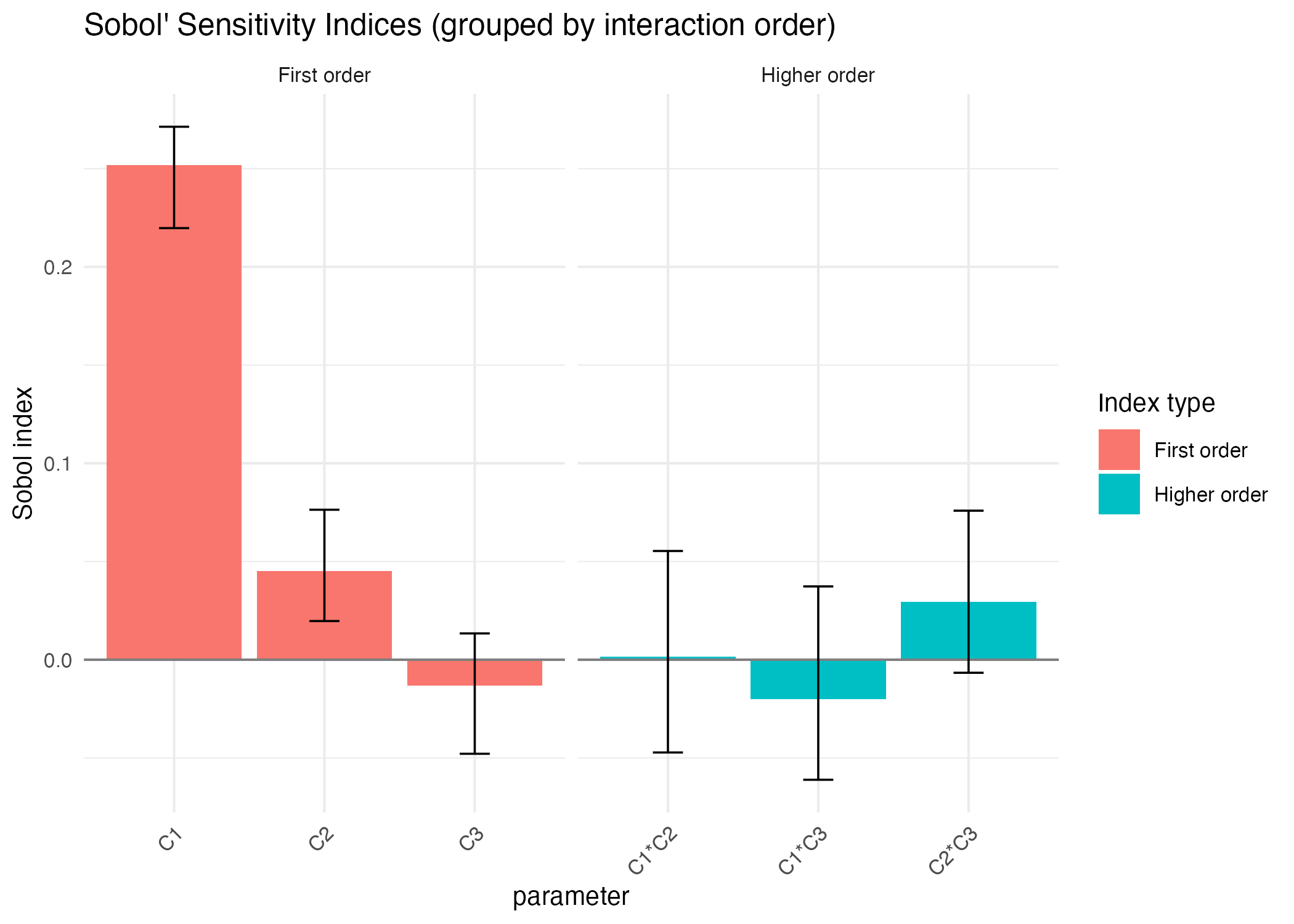
Order 1 and Total via sensitivity::sobol2007()
sob_cov_qoi <- sobol4r_qoi_indices(
  model = sobol_g2_with_covariate_noise,
  X1    = X1_cov,
  X2    = X2_cov,
  nboot = 50,
  type = "sobol2007")
print(sob_cov_qoi)
#>
#> Call:
#> sensitivity::sobol2007(model = NULL, X1 = X1, X2 = X2, nboot = nboot)
#>
#> Model runs: 50000
#>
#> First order indices:
#>        original          bias   std. error     min. c.i.    max. c.i.
#> C1 0.0003628503 -4.418472e-05 0.0002554395 -0.0001224899 0.0008875878
#> C2 0.0001646244  6.080073e-07 0.0001352320 -0.0001857294 0.0004557450
#> C3 0.9961673645  8.634919e-04 0.0198365066  0.9575067469 1.0521474300
#>
#> Total indices:
#>        original          bias   std. error     min. c.i.    max. c.i.
#> C1 0.0006914089 -5.703669e-05 0.0002709640  0.0002575406 0.0012294616
#> C2 0.0000394737  2.425451e-05 0.0001823106 -0.0005339253 0.0002984852
#> C3 1.0033002332  1.159900e-03 0.0119244876  0.9775140354 1.0294582460
Sobol4R::autoplot(sob_cov_qoi)