Sobol4R, Sobol Indices for Models with Fixed and Stochastic Parameters

Frédéric Bertrand, Elizaveta Logosha and Myriam Maumy-Bertrand

Tools to design experiments, compute Sobol sensitivity indices, and summarise stochastic responses inspired by the strategy described by Zhu et Sudret (2021) https://doi.org/10.1016/j.ress.2021.107815. Includes helpers to optimise toy models implemented in C++, visualise indices with uncertainty quantification, and derive reliability-oriented sensitivity measures based on failure probabilities. It is further detailed in Logosha, Maumy and Bertrand (2022) https://doi.org/10.1063/5.0246026 and (2023) https://doi.org/10.1063/5.0246024 or in Bertrand, Logosha and Maumy (2024) https://hal.science/hal-05371803, https://hal.science/hal-05371795 and https://hal.science/hal-05371798.

This site was created by F. Bertrand and the examples reproduced on it were created by F. Bertrand, E. Logosha and M. Maumy.

Installation

You can install the latest version of the Sobol4R package from github with:

devtools::install_github("fbertran/Sobol4R")

Two complementary analysis paths

Sobol4R exposes two ways to compute sensitivity indices depending on your workflow:

• Reuse the sensitivity package estimators. Provide pre-built designs and call sensitivity::sobol() or sensitivity::sobol2007(); the autoplot() methods in Sobol4R will visualise those results without changing your existing code.
• Use the in-package Saltelli re-implementation. The sobol_design() and sobol_indices() helpers build the matrices, run the model, and return a sobol_result object that can be summarised or plotted directly, with optional bootstrap quantiles for noisy simulations.

Two complementary analysis paths

Sobol4R exposes two ways to compute global sensitivity indices, depending on your workflow and the level of control you require.

• Use the in-package estimators with built-in Jansen support. The streamlined sobol_design() and sobol_indices() helpers generate the Saltelli-type matrices, evaluate the model (including replicated runs for stochastic simulators), and return a unified sobol_result object. Sobol4R implements several estimators internally, including Jansen, Martinez and Saltelli. The default estimator is Jansen, chosen for its numerical robustness and stable behaviour with non centred or noisy outputs. Results can be summarised or plotted directly and may include bootstrap quantiles when analysing stochastic simulators.

• Reuse the estimators from the sensitivity package. You can generate designs with Sobol4R (or your own routines) and pass the matrices directly to sensitivity::sobol(), sensitivity::sobol2007(), sensitivity::soboljansen(), sensitivity::sobolEff(), or sensitivity::sobolmartinez(). Sobol4R provides autoplot() methods that visualise these objects without altering your existing code.

Estimator defaults

The sobol4r_design(), sobol4r_run(), and sobol4r_qoi_indices() helpers mirror the sensitivity estimators: sobol, sobol2007, soboljansen, sobolEff, and sobolmartinez. They default to soboljansen because it is a numerically robust choice for both deterministic and stochastic simulators. A reasonable ordering for general-purpose work is:

1. soboljansen – stable first and total order indices, variance of differences, and broadly used in the literature.
2. sobolEff – efficient and well behaved, but a little more specialised than Jansen.
3. sobolmartinez – robust, though less common in practice.
4. sobol / sobol2007 – retained for backward compatibility with the original Saltelli-style estimators; they are less suited as defaults unless you explicitly centre outputs and control the setup.

The README examples below demonstrate the second path, while the earlier “Context and non random case” section illustrates interoperability with sensitivity.

Motivation

The methodology implemented in Sobol4R builds upon the stochastic Sobol analysis described by Lebrun et al. (2021) in Reliability Engineering & System Safety. The paper proposes to combine replicated simulator runs with Sobol estimators to account for intrinsic noise. The package mirrors this workflow:

1. Generate two Monte Carlo designs (A and B matrices).
2. Evaluate the stochastic simulator several times to estimate the mean response and the noise variance.
3. Derive first-order and total-order Sobol indices and visualise the results.

The package is also friendly with the sensitivity package and shows how to use the Sobol’ indices estimators provided in this package to increase the capabilities of this Sobol4R package.

Basic usage

library(Sobol4R)
set.seed(123)
design <- sobol_design(n = 256, d = 3, lower = rep(-pi, 3), upper = rep(pi, 3),
                       quasi = TRUE)
result <- sobol_indices(ishigami_model, design, replicates = 4,
                        keep_samples = TRUE)
result$data
#>   parameter first_order  total_order
#> 1        X1   0.4613292 4.263399e-05
#> 2        X2   0.8036762 3.506136e-01
#> 3        X3   0.6494604 1.963439e-01

The resulting object stores the Monte Carlo variance estimate, the average noise variance across replications, and the Sobol indices. Diagnostic plots are available through the provided autoplot() method:

autoplot(result)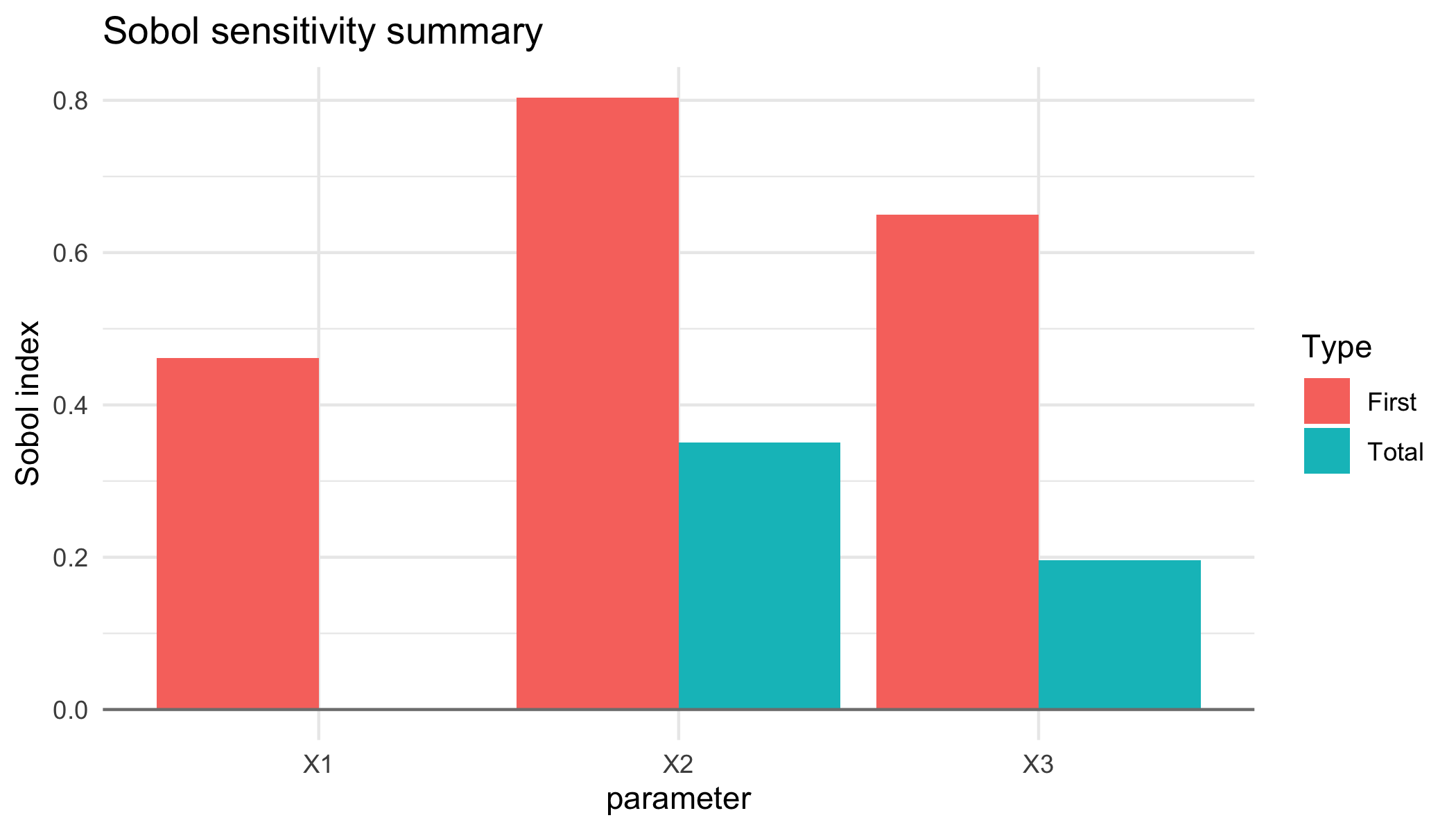

plot of chunk unnamed-chunk-3

When keep_samples = TRUE, bootstrap resamples quantify the estimator uncertainty. The helper summarise_sobol() produces tidy quantiles that can be visualised directly:

autoplot(result, show_uncertainty = TRUE, probs = c(0.1, 0.9), bootstrap = 100)

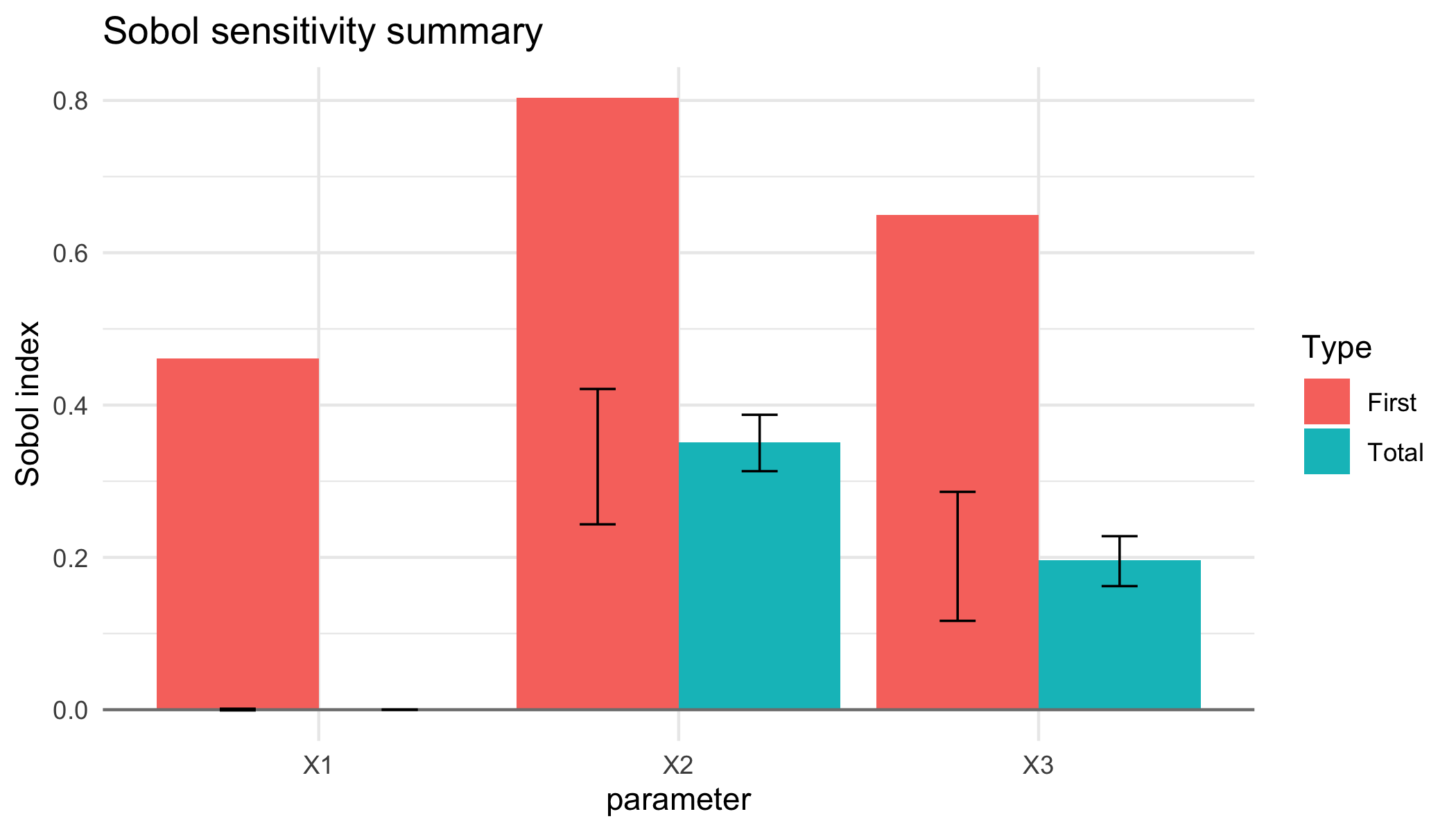
plot of chunk unnamed-chunk-4

Consistency check with the sensitivity estimators on Ishigami

The package exposes two ways to estimate Sobol indices: the in-package Saltelli implementation (sobol_indices()) and the sensitivity package estimators through sobol4r_design(). When comparing both, make sure the samples live on the correct domain of the simulator. The Ishigami benchmark expects ([-, ]) inputs; using the default ([0, 1]) cube would distort the indices and create spurious discrepancies.

library(Sobol4R)

set.seed(123)
design <- sobol_design(
  n     = 512,
  d     = 3,
  lower = rep(-pi, 3),
  upper = rep(pi, 3),
  quasi = TRUE
)

sobol4r_result <- sobol_indices(ishigami_model, design, replicates = 1)

sens_design <- sobol4r_design(
  X1 = as.data.frame(design$A),
  X2 = as.data.frame(design$B),
  order = 1,
  type = "sobol2007"
)
sens_output <- sensitivity::tell(sens_design, ishigami_model(as.matrix(sens_design$X)))

cbind(S_Sobol4R = sobol4r_result$data$first_order,
      T_Sobol4R = sobol4r_result$data$first_order, 
      S_sobol2007 = sens_output$S, 
      T_sobol2007 = sens_output$T) 
#>    S_Sobol4R T_Sobol4R     original      original
#> X1 0.2120769 0.2120769 0.0001129205 -6.480656e-05
#> X2 0.6454254 0.6454254 0.4415467860  4.338937e-01
#> X3 0.5724272 0.5724272 0.3770367118  3.499661e-01

Both estimators now report matching first-order and total-order indices for the Ishigami function because they rely on the same ([-, ]) inputs.

Reliability metrics

The paper highlights the need to quantify failure probabilities associated with critical performance levels. The package exposes a helper for that task:

set.seed(321)
simulated <- ishigami_model(matrix(runif(3000, -pi, pi), ncol = 3))
estimate_failure_probability(simulated, threshold = -1)
#> $probability
#> [1] 0.087
#> 
#> $variance
#> [1] 7.9431e-05

When the simulator is stochastic and sobol_indices() stores the replicated samples (keep_samples = TRUE), the same Monte Carlo budget can be recycled to derive failure-indicator Sobol indices:

failure <- sobol_reliability(result, threshold = -1)
failure$failure_probability
#> [1] 0.08984375
autoplot(failure, show_uncertainty = TRUE, probs = c(0.1, 0.9), bootstrap = 200)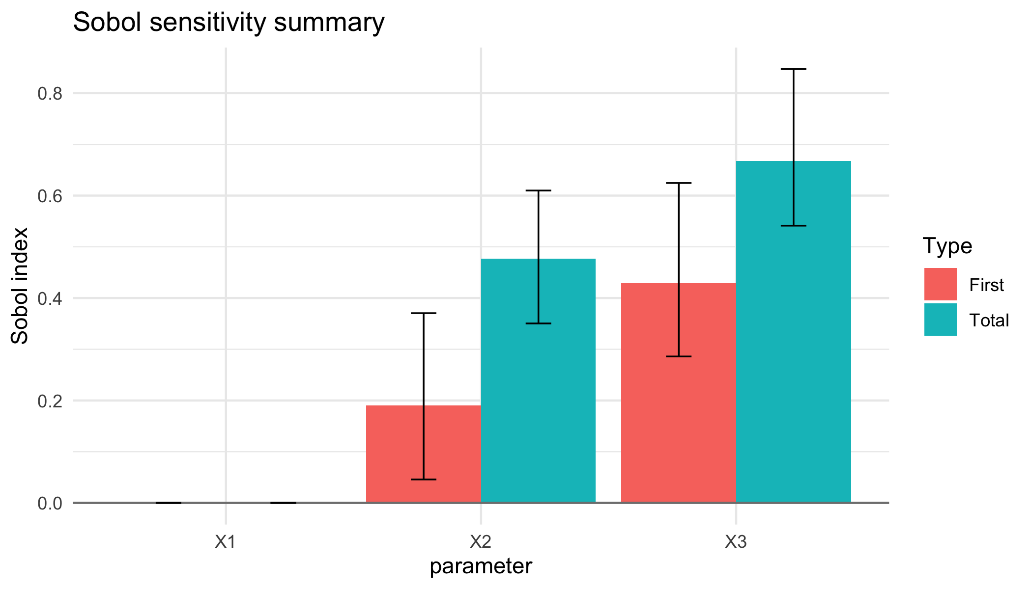

plot of chunk unnamed-chunk-7

Combined usage with the sensitivity package

Test case : the non-monotonic Sobol g-function

The method of Sobol requires two samples. In this reference case there are eight variables, all following the uniform distribution on $[0,1]$.

if(require(sensitivity)){
n <- 50000
p <- 8
X1_1 <- data.frame(matrix(runif(p * n), nrow = n))
X2_1 <- data.frame(matrix(runif(p * n), nrow = n))
}

if(require(sensitivity)){
set.seed(4669)
gensol1 <- sobol4r_design(
  X1    = X1_1,
  X2    = X2_1,
  order = 2,
  nboot = 100
)

Y1 <- sobol_g_function(gensol1$X)
x1 <- sensitivity::tell(gensol1, Y1)
print(x1)
}
#> 
#> Call:
#> sensitivity::soboljansen(model = NULL, X1 = X1, X2 = X2, nboot = nboot)
#> 
#> Model runs: 500000 
#> 
#> First order indices:
#>         original         bias  std. error
#> X1  7.158762e-01 0.0003292708 0.002812138
#> X2  1.788848e-01 0.0002168606 0.007105269
#> X3  2.477209e-02 0.0005654484 0.006774502
#> X4  6.589111e-03 0.0004831405 0.006838746
#> X5 -1.211742e-04 0.0005313759 0.006681976
#> X6  3.030053e-04 0.0005629356 0.006669775
#> X7  1.020259e-05 0.0005726937 0.006679191
#> X8  2.148300e-04 0.0005568268 0.006667389
#>       min. c.i.  max. c.i.
#> X1  0.710251368 0.72240556
#> X2  0.163947268 0.19201201
#> X3  0.009567471 0.03720730
#> X4 -0.008588815 0.01938342
#> X5 -0.015365761 0.01157217
#> X6 -0.015078821 0.01199152
#> X7 -0.015407550 0.01182783
#> X8 -0.015109380 0.01171543
#> 
#> Total indices:
#>        original          bias   std. error
#> X1 0.7935715807  7.383122e-05 5.720433e-03
#> X2 0.2415268270 -2.515680e-04 2.236182e-03
#> X3 0.0346698446  2.384117e-05 3.501189e-04
#> X4 0.0104714634  1.848957e-05 9.239132e-05
#> X5 0.0001052321 -2.571588e-08 9.742721e-07
#> X6 0.0001040942  1.012299e-07 1.107125e-06
#> X7 0.0001055571  8.766826e-08 8.914437e-07
#> X8 0.0001050610 -4.257143e-08 1.135505e-06
#>       min. c.i.    max. c.i.
#> X1 0.7816440833 0.8050569537
#> X2 0.2375455362 0.2463777104
#> X3 0.0340534615 0.0355355888
#> X4 0.0102682431 0.0106360252
#> X5 0.0001033743 0.0001069438
#> X6 0.0001021112 0.0001067899
#> X7 0.0001034028 0.0001068167
#> X8 0.0001028082 0.0001069985

if(require(sensitivity)){
autoplot(x1, ncol = 1)
}

plot of chunk det-g-plot

You can also use the sobol_example_g_deterministic() wrapper for this example.

if(require(sensitivity)){ex1_results <- sobol_example_g_deterministic()
print(ex1_results)
}
#> 
#> Call:
#> sensitivity::soboljansen(model = NULL, X1 = X1, X2 = X2, nboot = nboot)
#> 
#> Model runs: 500000 
#> 
#> First order indices:
#>        original          bias  std. error
#> X1  0.711999848  2.759449e-05 0.002631360
#> X2  0.171069444 -3.243317e-04 0.006964257
#> X3  0.019197160  2.380097e-04 0.006570602
#> X4  0.004399632  6.982094e-05 0.006591532
#> X5 -0.001721617  2.932782e-05 0.006368456
#> X6 -0.001881114  5.734953e-05 0.006392574
#> X7 -0.002045248  6.137792e-05 0.006369883
#> X8 -0.001850079  3.301663e-05 0.006399314
#>       min. c.i.  max. c.i.
#> X1  0.707005109 0.71676704
#> X2  0.156977789 0.18629660
#> X3  0.005519545 0.03206075
#> X4 -0.009336102 0.01681319
#> X5 -0.014976702 0.01081698
#> X6 -0.015225964 0.01075163
#> X7 -0.015444700 0.01055871
#> X8 -0.015159481 0.01093466
#> 
#> Total indices:
#>        original          bias   std. error
#> X1 0.7904857363  4.208462e-04 6.178943e-03
#> X2 0.2444730973  2.926195e-04 2.151611e-03
#> X3 0.0340828543  4.398558e-05 3.338495e-04
#> X4 0.0103959879 -3.029215e-06 8.915942e-05
#> X5 0.0001065903  1.171617e-07 9.079141e-07
#> X6 0.0001057113  1.810632e-07 9.735431e-07
#> X7 0.0001059162 -3.643364e-08 9.103740e-07
#> X8 0.0001042162  4.693930e-08 9.855479e-07
#>       min. c.i.    max. c.i.
#> X1 0.7787869014 0.8025046920
#> X2 0.2399293818 0.2482734385
#> X3 0.0334363304 0.0347126444
#> X4 0.0102354937 0.0105765331
#> X5 0.0001045168 0.0001082466
#> X6 0.0001037793 0.0001075022
#> X7 0.0001040602 0.0001081730
#> X8 0.0001021336 0.0001062003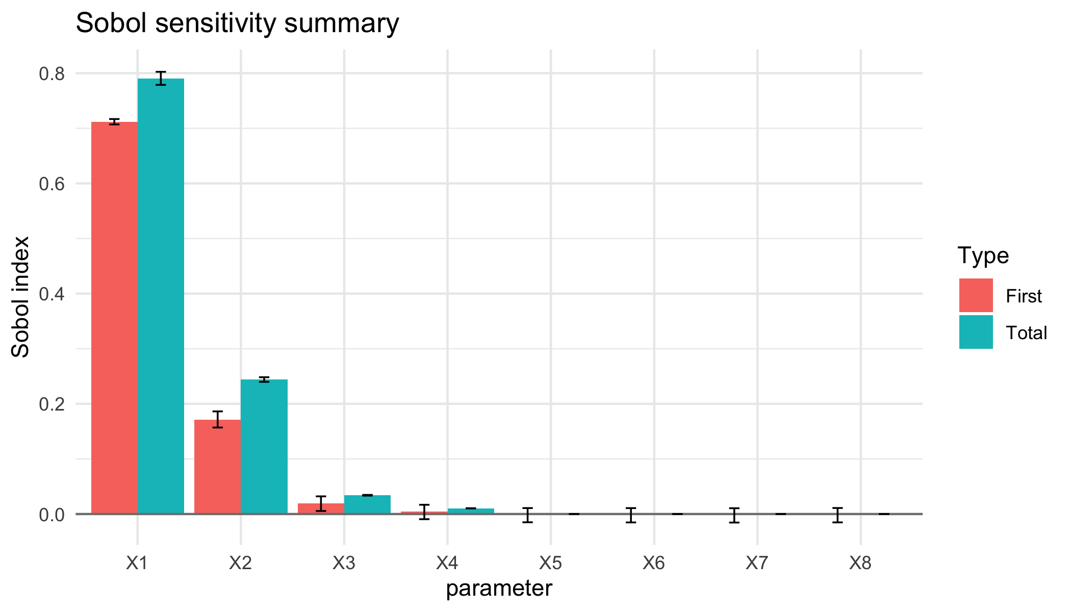

if(require(sensitivity)){
autoplot(ex1_results, ncol = 1)
}

plot of chunk unnamed-chunk-10

Vignettes

There are more insights and examples in the vignettes.

vignette("Sobol_RV_five_examples", package = "Sobol4R")
vignette("Sobol4R_vignette_stochastic", package = "Sobol4R")
vignette("Sobol4R_vignette_process", package = "Sobol4R")
vignette("simmer_MM1_Sobol_example", package = "Sobol4R")