Sobol sensitivity analysis of an M/M/1 queue in simmer

Model description

We consider a simple M/M/1 queue simulated with the simmer package.
Two input parameters are uncertain

lambda arrival rate (interarrival times distributed as Exp(lambda))
mu service rate (service times distributed as Exp(mu))

We study the impact of these two parameters on the mean waiting time in the queue at stationarity using Sobol indices.

Simulation model

# M/M/1 simmer model for Sobol analysis using time in system as QoI

library(simmer)
# One replication: mean time in system (sojourn time)
simulate_mm1_once_ts <- function(lambda, mu,
                                 horizon = 1000,
                                 warmup  = 200) {
  traj <- trajectory("customer") %>%
    seize("server") %>%
    timeout(function() rexp(1, rate = mu)) %>%
    release("server")
  
  env <- simmer("MM1_queue") %>%
    add_resource("server", capacity = 1, queue_size = Inf) %>%
    add_generator(
      name_prefix  = "cust",
      trajectory   = traj,
      distribution = function() rexp(1, rate = lambda)
    )
  
  env <- run(env, until = horizon)
  arr <- get_mon_arrivals(env)
  
  # Keep only post warmup
  arr <- arr[arr$end_time > warmup, , drop = FALSE]
  
  if (nrow(arr) == 0L) {
    return(0)
  }
  
  # Time in system = end_time - start_time
  ts <- arr$end_time - arr$start_time
  
  m <- mean(ts, na.rm = TRUE)
  if (!is.finite(m)) m <- 0
  m
}

# Quick sanity check
simulate_mm1_once_ts(lambda = 1/5, mu = 1/4)
#> [1] 11.99866

To reduce Monte Carlo noise, we define a quantity of interest (QoI) equal to the mean waiting time over several independent replications for the same parameter pair (lambda, mu).


# QoI: average mean time in system over replications
simulate_mm1_qoi_ts <- function(lambda, mu,
                                horizon = 1000,
                                warmup  = 200,
                                nrep   = 20L) {
  nrep <- as.integer(nrep)
  if (nrep < 1L) stop("'nrep' must be at least 1")
  vals <- replicate(
    nrep,
    simulate_mm1_once_ts(lambda = lambda, mu = mu,
                         horizon = horizon, warmup = warmup)
  )
  mean(vals)
}

simulate_mm1_qoi_ts(lambda = 1/5, mu = 1/4)
#> [1] 20.65865

Sobol model wrapper

The Sobol routine expects a model that takes a design matrix X and returns a numeric vector of length nrow(X). Here X has two columns

lambda
mu

# Model wrapper for sensitivity::sobol
mm1_sobol4r_model_ts <- function(X,
                               horizon = 1000,
                               warmup  = 200,
                               nrep   = 20L) {
  X <- as.data.frame(X)
  apply(X, 1L, function(par) {
    lambda <- par[1]
    mu     <- par[2]
    val <- simulate_mm1_qoi_ts(lambda = lambda, mu = mu,
                               horizon = horizon,
                               warmup  = warmup,
                               nrep   = nrep)
    if (!is.finite(val)) val <- 0
    val
  })
}

Sobol design for lambda and mu

We assume independent uniform priors

lambda in [0.10, 0.30]
mu in [0.20, 0.60]

n <- 200

X1 <- data.frame(
  lambda = runif(n, min = 0.10, max = 0.30),
  mu     = runif(n, min = 0.20, max = 0.60)
)

X2 <- data.frame(
  lambda = runif(n, min = 0.10, max = 0.30),
  mu     = runif(n, min = 0.20, max = 0.60)
)

# Helper to build a design region with non trivial queues but stable system
# choose lambda < mu, with rho close to 1
example_design_mm1_ts <- function(n = 100) {
  lambda <- runif(n, min = 0.18, max = 0.22)
  mu     <- runif(n, min = 0.23, max = 0.27)
  data.frame(lambda = lambda, mu = mu)
}

Sobol indices

library(simmer)
library(sensitivity)

set.seed(4669)

n  <- 150
X1 <- example_design_mm1_ts(n)
X2 <- example_design_mm1_ts(n)

sob_mm1 <- sobol(
  model = NULL,
  X1    = X1,
  X2    = X2,
  order = 2,
  nboot = 50
)

Y <- mm1_sobol4r_model_ts(
  sob_mm1$X,
  horizon = 1000,
  warmup  = 200,
  nrep   = 20
)

if (any(is.na(Y))) stop("Model returned NA values")
if (any(is.infinite(Y))) stop("Model returned infinite values")
summary(Y)             # should now show positive, variable values
#>    Min. 1st Qu.  Median    Mean 3rd Qu.    Max. 
#>   9.678  15.576  18.664  20.224  23.415  47.195
sob_mm1 <- tell(sob_mm1, Y)

print(sob_mm1)
#> 
#> Call:
#> sobol(model = NULL, X1 = X1, X2 = X2, order = 2, nboot = 50)
#> 
#> Model runs: 600 
#> 
#> Sobol indices
#>             original        bias std. error min. c.i. max. c.i.
#> lambda     0.8395726  0.17202798  0.5227109 -0.818910  1.539591
#> mu         0.8819571 -0.02622773  0.3794092 -0.303649  1.645314
#> lambda*mu -0.7266537 -0.15674237  0.6468889 -1.740781  1.107084

If ggplot2 is installed, we can visualise the indices with the autoplot method provided by the package.

Sobol4R::autoplot(sob_mm1)

Summary

We have shown how to

build a simple M/M/1 queue in simmer
define a scalar summary statistic (mean waiting time) as a QoI
wrap the simulator into a function compatible with sensitivity::sobol
compute Sobol indices for the two key parameters lambda and mu

The same pattern can be reused for more complex discrete event simulations implemented with simmer.

n <- 200
X1 <- data.frame(
  lambda = runif(n, 0.05, 0.20),
  mu_reg = runif(n, 0.30, 0.80),
  mu_exam = runif(n, 0.20, 0.60)
)
X2 <- data.frame(
  lambda = runif(n, 0.05, 0.20),
  mu_reg = runif(n, 0.30, 0.80),
  mu_exam = runif(n, 0.20, 0.60)
)

sob_clinic <- sobol(model = NULL,
                    X1    = X1,
                    X2    = X2,
                    order = 2,
                    nboot = 50)

Yc <- sobol4r_clinic_model(sob_clinic$X,
                           cap_reg = 2, 
                           cap_exam = 3,
                           horizon = 2000,
                           warmup_prob = 0.2,
                           nrep = 10)
sob_clinic <- tell(sob_clinic, Yc)
print(sob_clinic)
#> 
#> Call:
#> sobol(model = NULL, X1 = X1, X2 = X2, order = 2, nboot = 50)
#> 
#> Model runs: 1400 
#> 
#> Sobol indices
#>                   original        bias std. error  min. c.i. max. c.i.
#> lambda         -0.06917129 -0.01456138  0.4425323 -0.7768860 0.6526977
#> mu_reg          0.14549298  0.02817958  0.3568214 -0.6241805 0.8582114
#> mu_exam         0.94350070 -0.03795032  0.2581954  0.4647090 1.5558301
#> lambda*mu_reg   0.09415805  0.01032690  0.4447800 -0.6930579 0.7638910
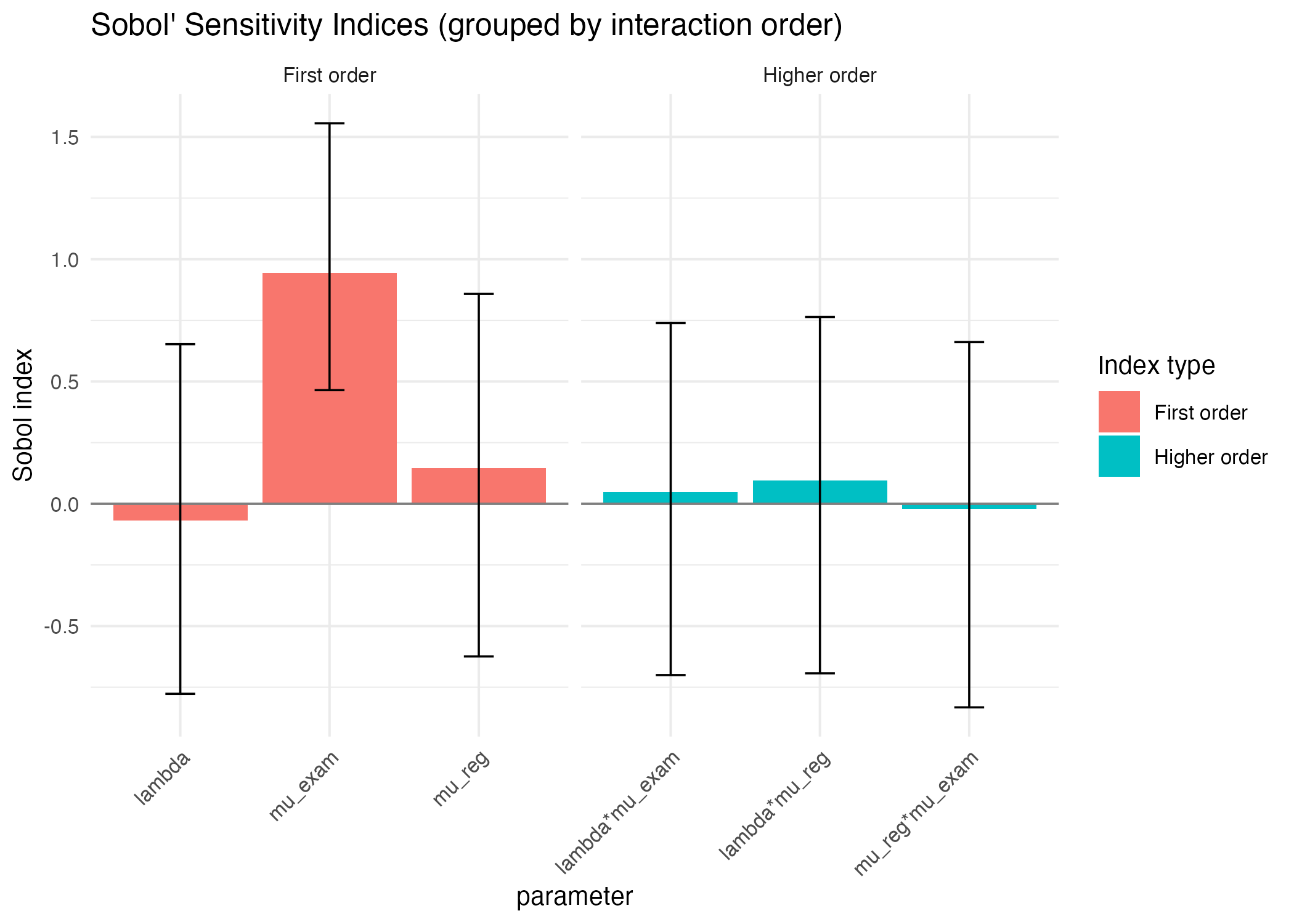
#> lambda*mu_exam  0.04811807  0.01390153  0.4365342 -0.7003076 0.7390800
#> mu_reg*mu_exam -0.02079743  0.01079563  0.4448869 -0.8323448 0.6611365
Sobol4R::autoplot(sob_clinic)