bootPLS, using bootstrap to find hyperparameters for Partial Least Squares Regression models and their extensions
Frédéric Bertrand, Jeremy Magnanensi and Myriam Maumy-Bertrand
https://doi.org/10.32614/CRAN.package.bootPLS
The goal of bootPLS is to provide several non-parametric stable bootstrap-based techniques to determine the numbers of components in Partial Least Squares and sparse Partial Least Squares linear or generalized linear regression.
bootPLS implements several algorithms that were published as a book chapter and two articles.
A new bootstrap-based stopping criterion in PLS component construction, J. Magnanensi, M. Maumy-Bertrand, N. Meyer and F. Bertrand (2016), in The Multiple Facets of Partial Least Squares and Related Methods. doi:10.1007/978-3-319-40643-5_18.
A new universal resample-stable bootstrap-based stopping criterion for PLS component construction, J. Magnanensi, F. Bertrand, M. Maumy-Bertrand and N. Meyer, (2017), Statistics and Computing, 27, 757–774. doi:10.1007/s11222-016-9651-4.
New developments in Sparse PLS regression, J. Magnanensi, M. Maumy-Bertrand, N. Meyer and F. Bertrand, (2021), Frontiers in Applied Mathematics and Statistics. doi:10.3389/fams.2021.693126.
Support for parallel computation and GPU is being developed.
This website and these examples were created by F. Bertrand and M. Maumy-Bertrand.
Installation
You can install the released version of bootPLS from CRAN with:
install.packages("bootPLS")You can install the development version of bootPLS from github with:
devtools::install_github("fbertran/bootPLS")Pine real dataset: pls and spls regressions
Loading and displaying dataset
Load and display the pinewood worm dataset.
library(bootPLS)
library(plsRglm)
data(pine, package = "plsRglm")
Xpine<-pine[,1:10]
ypine<-log(pine[,11])
pairs(pine)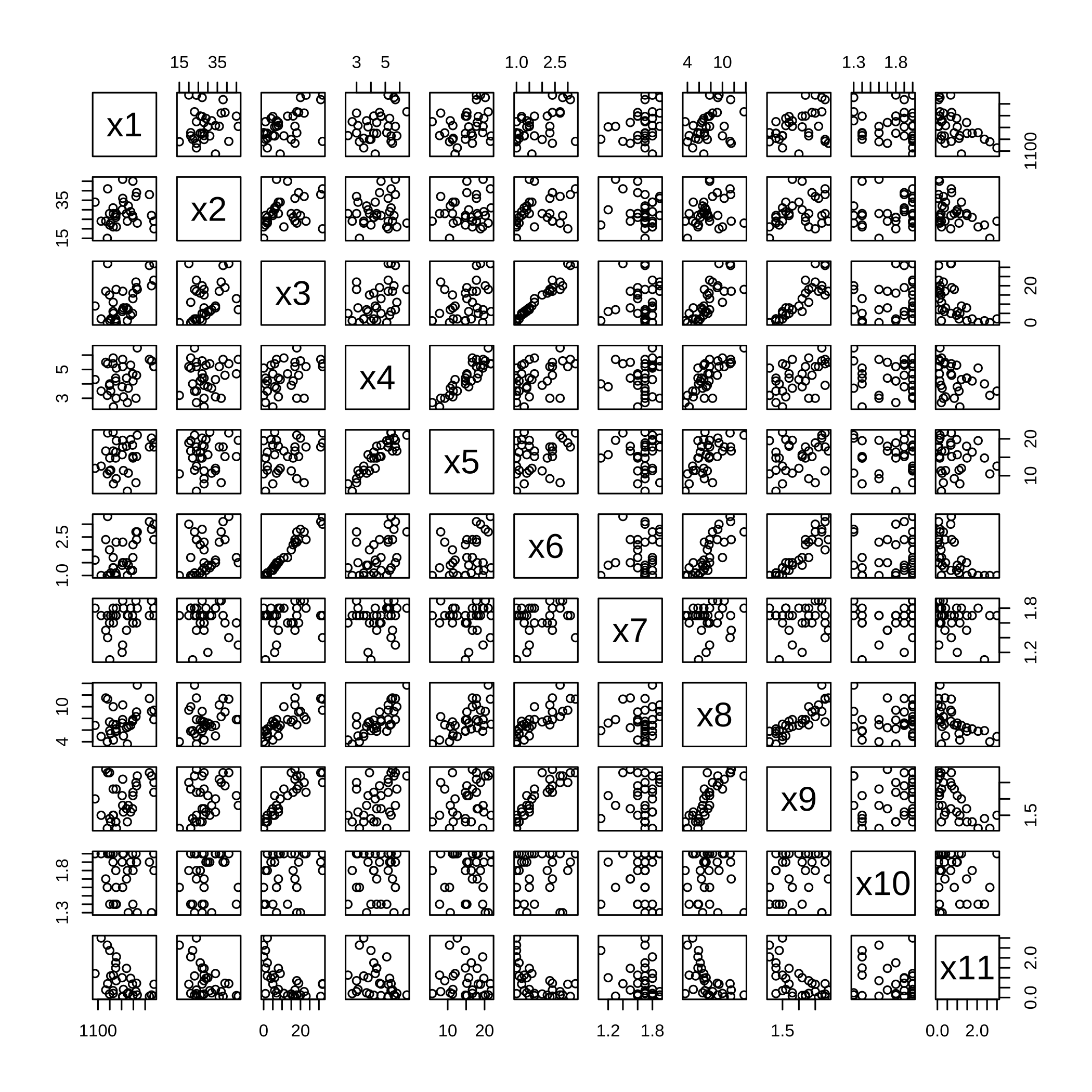
plot of chunk pinedisplay
Michel Tenenhaus’ reported in his book, La régression PLS (1998) Technip, Paris, that most of the expert biologists claimed that this dataset features two latent variables, which is tantamount to the PLS model having two components.
PLS LOO and CV
Leave one out CV (K=nrow(pine)) one time (NK=1).
bbb <- plsRglm::cv.plsR(log(x11)~.,data=pine,nt=6,K=nrow(pine),NK=1,verbose=FALSE)
plsRglm::cvtable(summary(bbb))
#> ____************************************************____
#> ____Component____ 1 ____
#> ____Component____ 2 ____
#> ____Component____ 3 ____
#> ____Component____ 4 ____
#> ____Component____ 5 ____
#> ____Component____ 6 ____
#> ____Predicting X without NA neither in X nor in Y____
#> Loading required namespace: plsdof
#> Error in loadNamespace(x): there is no package called 'plsdof'
Set up 6-fold CV (K=6), 100 times (NK=100), and use random=TRUE to randomly create folds for repeated CV.
Display the results of the cross-validation.
plsRglm::cvtable(summary(bbb2))
#> ____************************************************____
#> ____Component____ 1 ____
#> ____Component____ 2 ____
#> ____Component____ 3 ____
#> ____Component____ 4 ____
#> ____Component____ 5 ____
#> ____Component____ 6 ____
#> ____Predicting X without NA neither in X nor in Y____
#> Loading required namespace: plsdof
#> Error in loadNamespace(x): there is no package called 'plsdof'
The criterion is recommended in that PLSR setting without missing data. A model with 1 component is selected by the cross-validation as displayed by the following figure. Hence the criterion (1 component) does not agree with the experts (2 components).
plot(plsRglm::cvtable(summary(bbb2)),type="CVQ2")
#> ____************************************************____
#> ____Component____ 1 ____
#> ____Component____ 2 ____
#> ____Component____ 3 ____
#> ____Component____ 4 ____
#> ____Component____ 5 ____
#> ____Component____ 6 ____
#> ____Predicting X without NA neither in X nor in Y____
#> Loading required namespace: plsdof
#> Error in loadNamespace(x): there is no package called 'plsdof'
As for the CV Press criterion it is unable to point out a unique number of components.
plot(plsRglm::cvtable(summary(bbb2)),type="CVPress")
#> ____************************************************____
#> ____Component____ 1 ____
#> ____Component____ 2 ____
#> ____Component____ 3 ____
#> ____Component____ 4 ____
#> ____Component____ 5 ____
#> ____Component____ 6 ____
#> ____Predicting X without NA neither in X nor in Y____
#> Loading required namespace: plsdof
#> Error in loadNamespace(x): there is no package called 'plsdof'
PLS (Y,T) Bootstrap
The package features our bootstrap based algorithm to select the number of components in plsR regression. It is implemented with the nbcomp.bootplsR function.
set.seed(4619)
nbcomp.bootplsR(Y=ypine,X=Xpine,R =500)
#> [1] 1
#> ____************************************************____
#> ____Component____ 1 ____
#> ____Predicting X without NA neither in X nor in Y____
#> Loading required namespace: plsdof
#> Error in loadNamespace(x): there is no package called 'plsdof'
The verbose=FALSE option suppresses messages output during the algorithm, which is useful to replicate the bootstrap technique. To set up parallel computing, you can use the parallel and the ncpus options.
set.seed(4619)
res_boot_rep <- replicate(20,nbcomp.bootplsR(Y=ypine,X=Xpine,R =500,verbose =FALSE,parallel = "multicore",ncpus = 2))
#> Loading required namespace: plsdof
#> Error in loadNamespace(x): there is no package called 'plsdof'
It is easy to display the results with the barplot function.
A model with two components should be selected using our bootstrap based algorithm to select the number of components. Hence the number of component selected with our algorithm agrees with what was stated by the experts.
sPLS (Y,T) Bootstrap
The package also features our bootstrap based algorithm to select, for a given value, the number of components in spls regression. It is implemented with the nbcomp.bootspls function.
nbcomp.bootspls(x=Xpine,y=ypine,eta=.5)
#> eta = 0.5
#> [1] 1
#> [1] 2
#> [1] 3
#>
#> Optimal parameters: eta = 0.5, K = 2
plot of chunk nbcompbootspls
#> $mspemat
#>
#> eta= 0.5 , K= 2 1.187203
#>
#> $eta.opt
#> [1] 0.5
#>
#> $K.opt
#> [1] 2
A doParallel and foreach based parallel computing version of the algorithm is implemented as the nbcomp.bootspls.para function.
nbcomp.bootspls.para(x=Xpine,y=ypine,eta=.5)
#> [1] "eta = 0.5"
#> [1] 2
#> [1] 3
#>
#> Optimal parameters: eta = 0.5, K = 2
plot of chunk spls
#> $mspemat
#>
#> eta= 0.5 ; K= 2 1.085205
#>
#> $eta.opt
#> [1] 0.5
#>
#> $K.opt
#> [1] 2
nbcomp.bootspls.para(x=Xpine,y=ypine,eta=c(.2,.5))
#> [1] "eta = 0.2"
#> [1] 2
#> [1] 3
#> [1] "eta = 0.5"
#> [1] 2
#> [1] 3
#>
#> Optimal parameters: eta = 0.5, K = 2
plot of chunk spls
#> $mspemat
#>
#> eta= 0.2 ; K= 2 1.261797
#> eta= 0.5 ; K= 2 1.257117
#>
#> $eta.opt
#> [1] 0.5
#>
#> $K.opt
#> result.2
#>        2
Bootstrap (Y,X) for the coefficients with number of components updated for each resampling
Pinewood worm data reloaded.
library(bootPLS)
library(plsRglm)
data(pine, package = "plsRglm")
Xpine<-pine[,1:10]
ypine<-log(pine[,11])
datasetpine <- cbind(ypine,Xpine)
coefs.plsR.adapt.ncomp(datasetpine,sample(1:nrow(datasetpine)))
#> Loading required namespace: plsdof
#>  [1]  4.000000000 10.934323181 -0.004164703 -0.061586032
#>  [5]  0.038677103 -0.568792403  0.135567126  0.447111779
#>  [9] -0.885736030 -0.110684199 -1.141903333 -0.397050615
Replicate the results to get the bootstrap distributions of the selected number of components and the coefficients.
replicate(20,coefs.plsR.adapt.ncomp(datasetpine,sample(1:nrow(datasetpine))))
#>               [,1]         [,2]         [,3]         [,4]
#>  [1,]  2.000000000  2.000000000  2.000000000  2.000000000
#>  [2,]  8.064227044  8.064227044  8.064227044  8.064227044
#>  [3,] -0.003019447 -0.003019447 -0.003019447 -0.003019447
#>  [4,] -0.054389603 -0.054389603 -0.054389603 -0.054389603
#>  [5,] -0.005212285 -0.005212285 -0.005212285 -0.005212285
#>  [6,] -0.109946405 -0.109946405 -0.109946405 -0.109946405
#>  [7,]  0.038799785  0.038799785  0.038799785  0.038799785
#>  [8,] -0.078324545 -0.078324545 -0.078324545 -0.078324545
#>  [9,] -1.334080678 -1.334080678 -1.334080678 -1.334080678
#> [10,] -0.045021804 -0.045021804 -0.045021804 -0.045021804
#> [11,] -0.390730689 -0.390730689 -0.390730689 -0.390730689
#> [12,]  0.054696227  0.054696227  0.054696227  0.054696227
#>               [,5]         [,6]         [,7]         [,8]
#>  [1,]  2.000000000  2.000000000  2.000000000  2.000000000
#>  [2,]  8.064227044  8.064227044  8.064227044  8.064227044
#>  [3,] -0.003019447 -0.003019447 -0.003019447 -0.003019447
#>  [4,] -0.054389603 -0.054389603 -0.054389603 -0.054389603
#>  [5,] -0.005212285 -0.005212285 -0.005212285 -0.005212285
#>  [6,] -0.109946405 -0.109946405 -0.109946405 -0.109946405
#>  [7,]  0.038799785  0.038799785  0.038799785  0.038799785
#>  [8,] -0.078324545 -0.078324545 -0.078324545 -0.078324545
#>  [9,] -1.334080678 -1.334080678 -1.334080678 -1.334080678
#> [10,] -0.045021804 -0.045021804 -0.045021804 -0.045021804
#> [11,] -0.390730689 -0.390730689 -0.390730689 -0.390730689
#> [12,]  0.054696227  0.054696227  0.054696227  0.054696227
#>               [,9]        [,10]        [,11]        [,12]
#>  [1,]  2.000000000  2.000000000  2.000000000  2.000000000
#>  [2,]  8.064227044  8.064227044  8.064227044  8.064227044
#>  [3,] -0.003019447 -0.003019447 -0.003019447 -0.003019447
#>  [4,] -0.054389603 -0.054389603 -0.054389603 -0.054389603
#>  [5,] -0.005212285 -0.005212285 -0.005212285 -0.005212285
#>  [6,] -0.109946405 -0.109946405 -0.109946405 -0.109946405
#>  [7,]  0.038799785  0.038799785  0.038799785  0.038799785
#>  [8,] -0.078324545 -0.078324545 -0.078324545 -0.078324545
#>  [9,] -1.334080678 -1.334080678 -1.334080678 -1.334080678
#> [10,] -0.045021804 -0.045021804 -0.045021804 -0.045021804
#> [11,] -0.390730689 -0.390730689 -0.390730689 -0.390730689
#> [12,]  0.054696227  0.054696227  0.054696227  0.054696227
#>              [,13]        [,14]        [,15]        [,16]
#>  [1,]  2.000000000  2.000000000  2.000000000  2.000000000
#>  [2,]  8.064227044  8.064227044  8.064227044  8.064227044
#>  [3,] -0.003019447 -0.003019447 -0.003019447 -0.003019447
#>  [4,] -0.054389603 -0.054389603 -0.054389603 -0.054389603
#>  [5,] -0.005212285 -0.005212285 -0.005212285 -0.005212285
#>  [6,] -0.109946405 -0.109946405 -0.109946405 -0.109946405
#>  [7,]  0.038799785  0.038799785  0.038799785  0.038799785
#>  [8,] -0.078324545 -0.078324545 -0.078324545 -0.078324545
#>  [9,] -1.334080678 -1.334080678 -1.334080678 -1.334080678
#> [10,] -0.045021804 -0.045021804 -0.045021804 -0.045021804
#> [11,] -0.390730689 -0.390730689 -0.390730689 -0.390730689
#> [12,]  0.054696227  0.054696227  0.054696227  0.054696227
#>              [,17]        [,18]        [,19]        [,20]
#>  [1,]  2.000000000  2.000000000  2.000000000  2.000000000
#>  [2,]  8.064227044  8.064227044  8.064227044  8.064227044
#>  [3,] -0.003019447 -0.003019447 -0.003019447 -0.003019447
#>  [4,] -0.054389603 -0.054389603 -0.054389603 -0.054389603
#>  [5,] -0.005212285 -0.005212285 -0.005212285 -0.005212285
#>  [6,] -0.109946405 -0.109946405 -0.109946405 -0.109946405
#>  [7,]  0.038799785  0.038799785  0.038799785  0.038799785
#>  [8,] -0.078324545 -0.078324545 -0.078324545 -0.078324545
#>  [9,] -1.334080678 -1.334080678 -1.334080678 -1.334080678
#> [10,] -0.045021804 -0.045021804 -0.045021804 -0.045021804
#> [11,] -0.390730689 -0.390730689 -0.390730689 -0.390730689
#> [12,]  0.054696227  0.054696227  0.054696227  0.054696227
Parallel computing support with the ncpus and parallel="multicore" options.
coefs.plsR.adapt.ncomp(datasetpine,sample(1:nrow(datasetpine)),ncpus=2,parallel="multicore")
#>  [1]  2.000000000  8.064227044 -0.003019447 -0.054389603
#>  [5] -0.005212285 -0.109946405  0.038799785 -0.078324545
#>  [9] -1.334080678 -0.045021804 -0.390730689  0.054696227
replicate(20,coefs.plsR.adapt.ncomp(datasetpine,sample(1:nrow(datasetpine)),ncpus=2,parallel="multicore"))
#>               [,1]         [,2]         [,3]         [,4]
#>  [1,]  2.000000000  2.000000000  2.000000000  2.000000000
#>  [2,]  8.064227044  8.064227044  8.064227044  8.064227044
#>  [3,] -0.003019447 -0.003019447 -0.003019447 -0.003019447
#>  [4,] -0.054389603 -0.054389603 -0.054389603 -0.054389603
#>  [5,] -0.005212285 -0.005212285 -0.005212285 -0.005212285
#>  [6,] -0.109946405 -0.109946405 -0.109946405 -0.109946405
#>  [7,]  0.038799785  0.038799785  0.038799785  0.038799785
#>  [8,] -0.078324545 -0.078324545 -0.078324545 -0.078324545
#>  [9,] -1.334080678 -1.334080678 -1.334080678 -1.334080678
#> [10,] -0.045021804 -0.045021804 -0.045021804 -0.045021804
#> [11,] -0.390730689 -0.390730689 -0.390730689 -0.390730689
#> [12,]  0.054696227  0.054696227  0.054696227  0.054696227
#>               [,5]         [,6]         [,7]         [,8]
#>  [1,]  4.000000000  2.000000000  2.000000000  4.000000000
#>  [2,] 10.934323181  8.064227044  8.064227044 10.934323181
#>  [3,] -0.004164703 -0.003019447 -0.003019447 -0.004164703
#>  [4,] -0.061586032 -0.054389603 -0.054389603 -0.061586032
#>  [5,]  0.038677103 -0.005212285 -0.005212285  0.038677103
#>  [6,] -0.568792403 -0.109946405 -0.109946405 -0.568792403
#>  [7,]  0.135567126  0.038799785  0.038799785  0.135567126
#>  [8,]  0.447111779 -0.078324545 -0.078324545  0.447111779
#>  [9,] -0.885736030 -1.334080678 -1.334080678 -0.885736030
#> [10,] -0.110684199 -0.045021804 -0.045021804 -0.110684199
#> [11,] -1.141903333 -0.390730689 -0.390730689 -1.141903333
#> [12,] -0.397050615  0.054696227  0.054696227 -0.397050615
#>               [,9]        [,10]        [,11]        [,12]
#>  [1,]  2.000000000  2.000000000  2.000000000  2.000000000
#>  [2,]  8.064227044  8.064227044  8.064227044  8.064227044
#>  [3,] -0.003019447 -0.003019447 -0.003019447 -0.003019447
#>  [4,] -0.054389603 -0.054389603 -0.054389603 -0.054389603
#>  [5,] -0.005212285 -0.005212285 -0.005212285 -0.005212285
#>  [6,] -0.109946405 -0.109946405 -0.109946405 -0.109946405
#>  [7,]  0.038799785  0.038799785  0.038799785  0.038799785
#>  [8,] -0.078324545 -0.078324545 -0.078324545 -0.078324545
#>  [9,] -1.334080678 -1.334080678 -1.334080678 -1.334080678
#> [10,] -0.045021804 -0.045021804 -0.045021804 -0.045021804
#> [11,] -0.390730689 -0.390730689 -0.390730689 -0.390730689
#> [12,]  0.054696227  0.054696227  0.054696227  0.054696227
#>              [,13]        [,14]        [,15]        [,16]
#>  [1,]  2.000000000  2.000000000  2.000000000  2.000000000
#>  [2,]  8.064227044  8.064227044  8.064227044  8.064227044
#>  [3,] -0.003019447 -0.003019447 -0.003019447 -0.003019447
#>  [4,] -0.054389603 -0.054389603 -0.054389603 -0.054389603
#>  [5,] -0.005212285 -0.005212285 -0.005212285 -0.005212285
#>  [6,] -0.109946405 -0.109946405 -0.109946405 -0.109946405
#>  [7,]  0.038799785  0.038799785  0.038799785  0.038799785
#>  [8,] -0.078324545 -0.078324545 -0.078324545 -0.078324545
#>  [9,] -1.334080678 -1.334080678 -1.334080678 -1.334080678
#> [10,] -0.045021804 -0.045021804 -0.045021804 -0.045021804
#> [11,] -0.390730689 -0.390730689 -0.390730689 -0.390730689
#> [12,]  0.054696227  0.054696227  0.054696227  0.054696227
#>              [,17]        [,18]        [,19]        [,20]
#>  [1,]  2.000000000  2.000000000  2.000000000  2.000000000
#>  [2,]  8.064227044  8.064227044  8.064227044  8.064227044
#>  [3,] -0.003019447 -0.003019447 -0.003019447 -0.003019447
#>  [4,] -0.054389603 -0.054389603 -0.054389603 -0.054389603
#>  [5,] -0.005212285 -0.005212285 -0.005212285 -0.005212285
#>  [6,] -0.109946405 -0.109946405 -0.109946405 -0.109946405
#>  [7,]  0.038799785  0.038799785  0.038799785  0.038799785
#>  [8,] -0.078324545 -0.078324545 -0.078324545 -0.078324545
#>  [9,] -1.334080678 -1.334080678 -1.334080678 -1.334080678
#> [10,] -0.045021804 -0.045021804 -0.045021804 -0.045021804
#> [11,] -0.390730689 -0.390730689 -0.390730689 -0.390730689
#> [12,]  0.054696227  0.054696227  0.054696227  0.054696227
Aze real dataset: binary logistic plsRglm and sgpls regressions
PLSGLR (Y,T) Bootstrap
Loading the data and creating the data frames.
data(aze_compl)
Xaze_compl<-aze_compl[,2:34]
yaze_compl<-aze_compl$y
dataset <- cbind(y=yaze_compl,Xaze_compl)
Fitting a logistic PLS regression model with 10 components. You have to use the family option when fitting the plsRglm.
modplsglm <- plsRglm(y~.,data=dataset,10,modele="pls-glm-family",family="binomial")
#> ____************************************************____
#>
#> Family: binomial
#> Link function: logit
#>
#> ____Component____ 1 ____
#> ____Component____ 2 ____
#> ____Component____ 3 ____
#> ____Component____ 4 ____
#> ____Component____ 5 ____
#> ____Component____ 6 ____
#> ____Component____ 7 ____
#> ____Component____ 8 ____
#> ____Component____ 9 ____
#> ____Component____ 10 ____
#> ____Predicting X without NA neither in X or Y____
#> ****________________________________________________****
Perform the bootstrap based algorithm with the nbcomp.bootplsRglm function. By default 250 resamplings are carried out.
set.seed(4619)
aze_compl.bootYT <- suppressWarnings(nbcomp.bootplsRglm(modplsglm))
Plotting the bootstrap distributions of the coefficients of the components.
plsRglm::boxplots.bootpls(aze_compl.bootYT)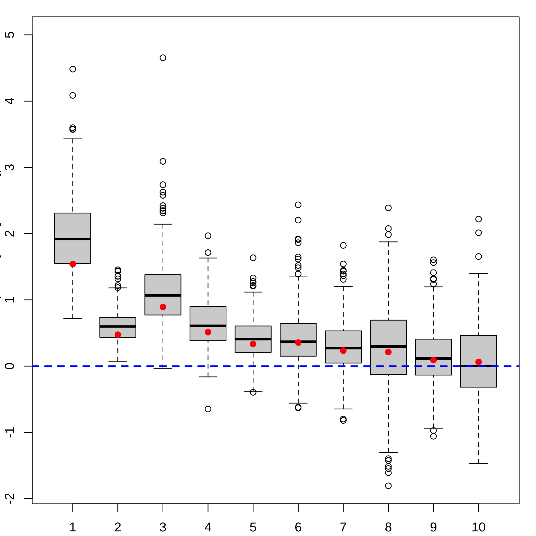
plot of chunk azeplotbootcomp
Computing the bootstrap based confidence intervals of the coefficients of the components.
plsRglm::confints.bootpls(aze_compl.bootYT)
#> Warning in norm.inter(t, adj.alpha): extreme order statistics used
#> as endpoints
#> Warning in norm.inter(t, adj.alpha): extreme order statistics used
#> as endpoints
#> Warning in norm.inter(t, adj.alpha): extreme order statistics used
#> as endpoints
#>
#>  [1,] -0.1909709 2.3581748 -0.4489036 1.9697388  1.11236461
#>  [2,] -0.1514302 0.8243332 -0.3376837 0.7471037  0.20267973
#>  [3,] -0.4319055 1.7434199 -0.6285256 1.5594694  0.22338048
#>  [4,] -0.3748813 1.0973698 -0.5490521 0.9657205  0.05733105
#>  [5,] -0.3963722 0.8830876 -0.5130832 0.8905919 -0.22108731
#>  [6,] -0.6441165 1.2480090 -0.9267788 1.1913771 -0.47946992
#>  [7,] -0.6863159 1.0264625 -0.8829492 1.0706084 -0.60361567
#>  [8,] -1.1970167 1.4738770 -1.2043483 1.7957092 -1.37023450
#>  [9,] -0.8340372 0.9057530 -1.0433636 0.9124285 -0.72858196
#> [10,] -1.0786394 1.2056122 -1.1600493 1.2398892 -1.11385399
#>
#>  [1,] 3.531007  0.71686088 2.1861124
#>  [2,] 1.287467  0.07412900 0.8286440
#>  [3,] 2.411375 -0.03355241 1.6424348
#>  [4,] 1.572104 -0.45493576 1.1619803
#>  [5,] 1.182588 -0.38904916 0.9004701
#>  [6,] 1.638686 -0.53350462 1.4582694
#>  [7,] 1.349942 -0.75368847 1.0112706
#>  [8,] 1.629823 -1.54876392 1.3140140
#>  [9,] 1.227210 -0.74456869 1.1516065
#> [10,] 1.286084 -1.02902293 1.3514701
#> attr(,"typeBCa")
#> [1] TRUE
Computing the bootstrap based confidence intervals of the coefficients of the components.
suppressWarnings(plsRglm::plots.confints.bootpls(plsRglm::confints.bootpls(aze_compl.bootYT)))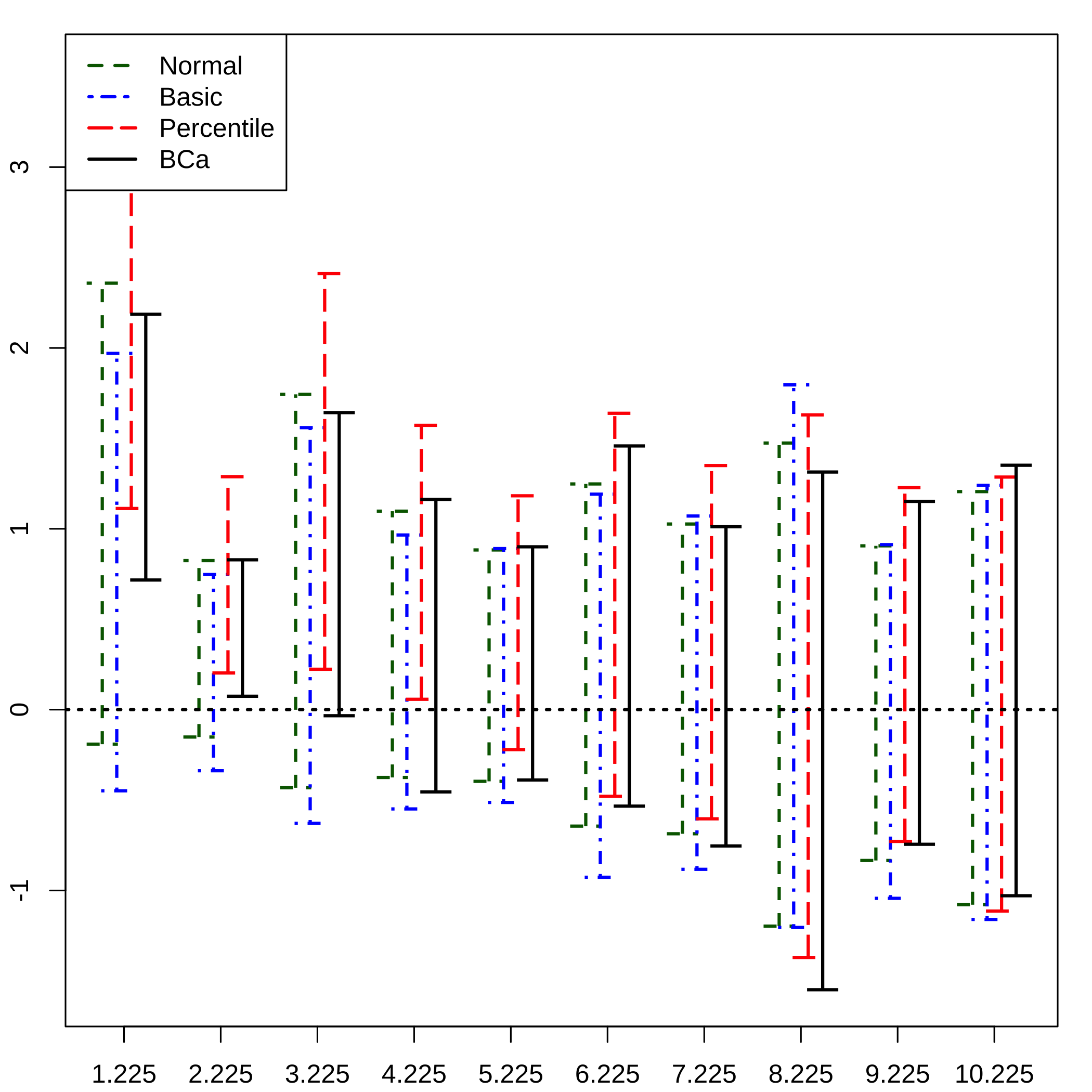
plot of chunk azebootcompplotCI
sparse PLSGLR (Y,T) Bootstrap
The package also features our bootstrap based algorithm to select, for a given value, the number of components in sgpls regression. It is implemented in the nbcomp.bootsgpls.
set.seed(4619)
data(prostate, package="spls")
nbcomp.bootsgpls((prostate$x)[,1:30], prostate$y, R=250, eta=0.2, typeBCa = FALSE)
#> [1] "eta = 0.2"
#> [1] "K = 1"
#> [1] "K = 2"
#> [1] "K = 3"
#> [1] "K = 4"
#> [1] "K = 5"
#> Warning: glm.fit: fitted probabilities numerically 0 or 1 occurred
#>
#> Optimal parameters: eta = 0.2, K = 4
plot of chunk prostateload
#> $err.mat
#>
#> eta= 0.2 ; K= 4 0.2554545
#>
#> $eta.opt
#> [1] 0.2
#>
#> $K.opt
#> [1] 4
#>
#> $cands
#>           [,1] [,2] [,3] [,4]
#> [1,] 0.2554545   30  0.2    4
A doParallel and foreach based parallel computing version of the algorithm is implemented as the nbcomp.bootspls.para function.
nbcomp.bootsgpls.para((prostate$x)[,1:30], prostate$y, R=250, eta=c(.2,.5), maxnt=10, typeBCa = FALSE)
#> [1] "eta = 0.2"
#> [1] "K = 1"
#> [1] "K = 2"
#> [1] "K = 3"
#> [1] "K = 4"
#> [1] "K = 5"
#> [1] "eta = 0.5"
#> [1] "K = 1"
#> [1] "K = 2"
#> [1] "K = 3"
#> [1] "K = 4"
#> [1] "K = 5"
#> Warning: glm.fit: algorithm did not converge
#> Warning: glm.fit: fitted probabilities numerically 0 or 1 occurred
#> Warning: glm.fit: fitted probabilities numerically 0 or 1 occurred
#> Warning: glm.fit: fitted probabilities numerically 0 or 1 occurred
#>
#> Optimal parameters: eta = 0.5, K = 4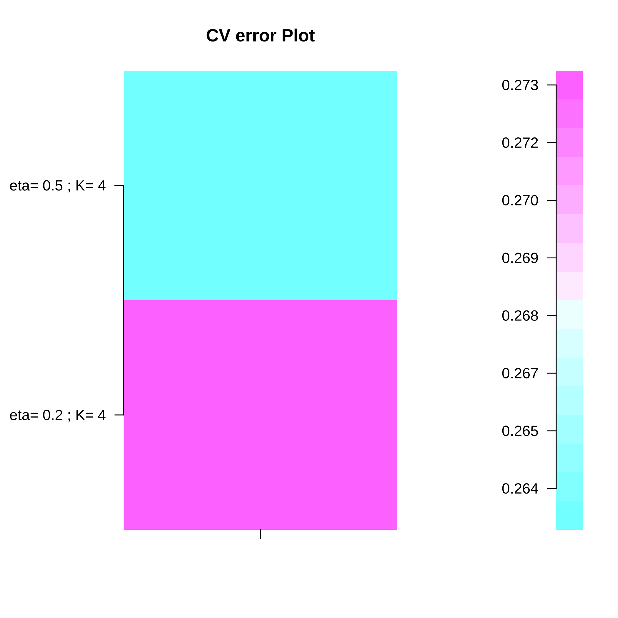
plot of chunk prostatespls
#> $err.mat
#>
#> eta= 0.2 ; K= 4 0.2727273
#> eta= 0.5 ; K= 4 0.2636364
#>
#> $eta.opt
#> [1] 0.5
#>
#> $K.opt
#> [1] 4
#>
#> $cands
#>           [,1] [,2] [,3] [,4]
#> [1,] 0.2636364 27.4  0.5    4