Partial least squares regression glm models with k-fold cross validation
cv.plsRglm.RdThis function implements k-fold cross-validation on complete or incomplete datasets for partial least squares regression generalized linear models
Usage
cv.plsRglm(object, ...)
# Default S3 method
cv.plsRglmmodel(object,dataX,nt=2,limQ2set=.0975,
modele="pls", family=NULL, K=5, NK=1, grouplist=NULL, random=TRUE,
scaleX=TRUE, scaleY=NULL, keepcoeffs=FALSE, keepfolds=FALSE,
keepdataY=TRUE, keepMclassed=FALSE, tol_Xi=10^(-12), weights, method,
fit_backend="stats",verbose=TRUE,...)
# S3 method for class 'formula'
cv.plsRglmmodel(object,data=NULL,nt=2,limQ2set=.0975,
modele="pls", family=NULL, K=5, NK=1, grouplist=NULL, random=TRUE,
scaleX=TRUE, scaleY=NULL, keepcoeffs=FALSE, keepfolds=FALSE,
keepdataY=TRUE, keepMclassed=FALSE, tol_Xi=10^(-12),weights,subset,
start=NULL,etastart,mustart,offset,method,control= list(),contrasts=NULL,
fit_backend="stats",verbose=TRUE,...)
PLS_glm_kfoldcv(dataY, dataX, nt = 2, limQ2set = 0.0975, modele = "pls",
family = NULL, K = 5, NK = 1, grouplist = NULL, random = TRUE,
scaleX = TRUE, scaleY = NULL, keepcoeffs = FALSE, keepfolds = FALSE,
keepdataY = TRUE, keepMclassed=FALSE, tol_Xi = 10^(-12), weights, method,
fit_backend="stats",verbose=TRUE)
PLS_glm_kfoldcv_formula(formula,data=NULL,nt=2,limQ2set=.0975,modele="pls",
family=NULL, K=5, NK=1, grouplist=NULL, random=TRUE,
scaleX=TRUE, scaleY=NULL, keepcoeffs=FALSE, keepfolds=FALSE, keepdataY=TRUE,
keepMclassed=FALSE, tol_Xi=10^(-12),weights,subset,start=NULL,etastart,
mustart,offset,method,control= list(),contrasts=NULL, fit_backend="stats",
verbose=TRUE)
Arguments
- object
response (training) dataset or an object of class "
formula" (or one that can be coerced to that class): a symbolic description of the model to be fitted. The details of model specification are given under 'Details'.- dataY
response (training) dataset
- dataX
predictor(s) (training) dataset
- formula
an object of class "
formula" (or one that can be coerced to that class): a symbolic description of the model to be fitted. The details of model specification are given under 'Details'.- data
an optional data frame, list or environment (or object coercible by
as.data.frameto a data frame) containing the variables in the model. If not found indata, the variables are taken fromenvironment(formula), typically the environment from whichplsRglmis called.- nt
number of components to be extracted
- limQ2set
limit value for the Q2
- modele
name of the PLS glm model to be fitted (
"pls","pls-glm-Gamma","pls-glm-gaussian","pls-glm-inverse.gaussian","pls-glm-logistic","pls-glm-poisson","pls-glm-polr"). Use"modele=pls-glm-family"to enable thefamilyoption.- family
a description of the error distribution and link function to be used in the model. This can be a character string naming a family function, a family function or the result of a call to a family function. (See
familyfor details of family functions.) To use the family option, please setmodele="pls-glm-family". User defined families can also be defined. See details.- K
number of groups. Defaults to 5.
- NK
number of times the group division is made
- grouplist
to specify the members of the
Kgroups- random
should the
Kgroups be made randomly. Defaults toTRUE- scaleX
scale the predictor(s) : must be set to TRUE for
modele="pls"and should be for glms pls.- scaleY
scale the response : Yes/No. Ignored since non always possible for glm responses.
- keepcoeffs
shall the coefficients for each model be returned
- keepfolds
shall the groups' composition be returned
- keepdataY
shall the observed value of the response for each one of the predicted value be returned
- keepMclassed
shall the number of miss classed be returned (unavailable)
- tol_Xi
minimal value for Norm2(Xi) and \(\mathrm{det}(pp' \times pp)\) if there is any missing value in the
dataX. It defaults to \(10^{-12}\)- weights
an optional vector of 'prior weights' to be used in the fitting process. Should be
NULLor a numeric vector.- fit_backend
backend used for repeated non-ordinal score-space GLM fits during cross-validation. Use
"stats"for the compatibility path or"fastglm"to opt into the accelerated complete-data backend. Unsupported cases fall back to"stats"with a warning.- subset
an optional vector specifying a subset of observations to be used in the fitting process.
- start
starting values for the parameters in the linear predictor.
- etastart
starting values for the linear predictor.
- mustart
starting values for the vector of means.
- offset
this can be used to specify an a priori known component to be included in the linear predictor during fitting. This should be
NULLor a numeric vector of length equal to the number of cases. One or moreoffsetterms can be included in the formula instead or as well, and if more than one is specified their sum is used. Seemodel.offset.- method
For non-ordinal GLM modes this argument is kept for backward compatibility; use
fit_backendto choose the score-space fitting backend. Forpls-glm-polr, uselogistic,probit, complementary log-log orcauchit.- control
a list of parameters for controlling the fitting process. For
glm.fitthis is passed toglm.control.- contrasts
an optional list. See the
contrasts.argofmodel.matrix.default.- verbose
should info messages be displayed ?
- ...
arguments to pass to
cv.plsRglmmodel.defaultor tocv.plsRglmmodel.formula
Details
Predicts 1 group with the K-1 other groups. Leave one out cross validation is thus obtained for K==nrow(dataX).
There are seven different predefined models with predefined link functions available :
"pls"ordinary pls models
"pls-glm-Gamma"glm gaussian with inverse link pls models
"pls-glm-gaussian"glm gaussian with identity link pls models
"pls-glm-inverse-gamma"glm binomial with square inverse link pls models
"pls-glm-logistic"glm binomial with logit link pls models
"pls-glm-poisson"glm poisson with log link pls models
"pls-glm-polr"glm polr with logit link pls models
Using the "family=" option and setting "modele=pls-glm-family" allows changing the family and link function the same way as for the glm function. As a consequence user-specified families can also be used.
- The
gaussianfamily accepts the links (as names)
identity,logandinverse.- The
binomialfamily accepts the links
logit,probit,cauchit, (corresponding to logistic, normal and Cauchy CDFs respectively)logandcloglog(complementary log-log).- The
Gammafamily accepts the links
inverse,identityandlog.- The
poissonfamily accepts the links
log,identity, andsqrt.- The
inverse.gaussianfamily accepts the links
1/mu^2,inverse,identityandlog.- The
quasifamily accepts the links
logit,probit,cloglog,identity,inverse,log,1/mu^2andsqrt.- The function
power can be used to create a power link function.
- ...
arguments to pass to
cv.plsRglmmodel.defaultor tocv.plsRglmmodel.formula
A typical predictor has the form response ~ terms where response is the (numeric) response vector and terms is a series of terms which specifies a linear predictor for response. A terms specification of the form first + second indicates all the terms in first together with all the terms in second with any duplicates removed.
A specification of the form first:second indicates the the set of terms obtained by taking the interactions of all terms in first with all terms in second. The specification first*second indicates the cross of first and second. This is the same as first + second + first:second.
The terms in the formula will be re-ordered so that main effects come first, followed by the interactions, all second-order, all third-order and so on: to avoid this pass a terms object as the formula.
Non-NULL weights can be used to indicate that different observations have different dispersions (with the values in weights being inversely proportional to the dispersions); or equivalently, when the elements of weights are positive integers w_i, that each response y_i is the mean of w_i unit-weight observations.
Value
An object of class "cv.plsRglmmodel".
- results_kfolds
list of
NK. Each element of the list sums up the results for a group division:- list
of
Kmatrices of size aboutnrow(dataX)/K * ntwith the predicted values for a growing number of components- ...
...
- list
of
Kmatrices of size aboutnrow(dataX)/K * ntwith the predicted values for a growing number of components
- folds
list of
NK. Each element of the list sums up the informations for a group division:- list
of
Kvectors of length aboutnrow(dataX)with the numbers of the rows ofdataXthat were used as a training set- ...
...
- list
of
Kvectors of length aboutnrow(dataX)with the numbers of the rows ofdataXthat were used as a training set
- dataY_kfolds
list of
NK. Each element of the list sums up the results for a group division:- list
of
Kmatrices of size aboutnrow(dataX)/K * 1with the observed values of the response- ...
...
- list
of
Kmatrices of size aboutnrow(dataX)/K * 1with the observed values of the response
- fit_backend
backend used for repeated non-ordinal score-space GLM fits during cross-validation
- call
the call of the function
References
Nicolas Meyer, Myriam Maumy-Bertrand et Frederic Bertrand (2010). Comparing the linear and the logistic PLS regression with qualitative predictors: application to allelotyping data. Journal de la Societe Francaise de Statistique, 151(2), pages 1-18.
Author
Frederic Bertrand
frederic.bertrand@lecnam.net
https://fbertran.github.io/homepage/
See also
Summary method summary.cv.plsRglmmodel. kfolds2coeff, kfolds2Pressind, kfolds2Press, kfolds2Mclassedind, kfolds2Mclassed and summary to extract and transform results from k-fold cross validation.
Examples
data(Cornell)
bbb <- cv.plsRglm(Y~.,data=Cornell,nt=10)
#>
#> Model: pls
#>
#> NK: 1
#> Number of groups : 5
#> 1
#> ____************************************************____
#>
#> Model: pls
#>
#> ____Predicting X without NA neither in X nor in Y____
#> ____Component____ 1 ____
#> ____Component____ 2 ____
#> ____Component____ 3 ____
#> ____Component____ 4 ____
#> ____Component____ 5 ____
#> ____Component____ 6 ____
#> Warning : < 10^{-12}
#> Warning only 6 components could thus be extracted
#> ****________________________________________________****
#>
#> 2
#> ____************************************************____
#>
#> Model: pls
#>
#> ____Predicting X without NA neither in X nor in Y____
#> ____Component____ 1 ____
#> ____Component____ 2 ____
#> ____Component____ 3 ____
#> ____Component____ 4 ____
#> ____Component____ 5 ____
#> ____Component____ 6 ____
#> Warning : < 10^{-12}
#> Warning only 6 components could thus be extracted
#> ****________________________________________________****
#>
#> 3
#> ____************************************************____
#>
#> Model: pls
#>
#> ____Predicting X without NA neither in X nor in Y____
#> ____Component____ 1 ____
#> ____Component____ 2 ____
#> ____Component____ 3 ____
#> ____Component____ 4 ____
#> ____Component____ 5 ____
#> Warning : < 10^{-12}
#> Warning only 5 components could thus be extracted
#> ****________________________________________________****
#>
#> 4
#> ____************************************************____
#>
#> Model: pls
#>
#> ____Predicting X without NA neither in X nor in Y____
#> ____Component____ 1 ____
#> ____Component____ 2 ____
#> ____Component____ 3 ____
#> ____Component____ 4 ____
#> ____Component____ 5 ____
#> ____Component____ 6 ____
#> Warning : < 10^{-12}
#> Warning only 6 components could thus be extracted
#> ****________________________________________________****
#>
#> 5
#> ____************************************************____
#>
#> Model: pls
#>
#> ____Predicting X without NA neither in X nor in Y____
#> ____Component____ 1 ____
#> ____Component____ 2 ____
#> ____Component____ 3 ____
#> ____Component____ 4 ____
#> ____Component____ 5 ____
#> ____Component____ 6 ____
#> Warning : < 10^{-12}
#> Warning only 6 components could thus be extracted
#> ****________________________________________________****
#>
(sum1<-summary(bbb))
#> ____************************************************____
#>
#> Model: pls
#>
#> ____Component____ 1 ____
#> ____Component____ 2 ____
#> ____Component____ 3 ____
#> ____Component____ 4 ____
#> ____Component____ 5 ____
#> ____Component____ 6 ____
#> ____Predicting X without NA neither in X or Y____
#> ****________________________________________________****
#>
#>
#> NK: 1
#> [[1]]
#> AIC Q2cum_Y LimQ2_Y Q2_Y PRESS_Y RSS_Y R2_Y
#> Nb_Comp_0 82.01205 NA NA NA NA 467.796667 NA
#> Nb_Comp_1 53.15173 0.8625059 0.0975 0.8625059 64.31930 35.742486 0.9235940
#> Nb_Comp_2 41.08283 0.8328694 0.0975 -0.2155470 43.44667 11.066606 0.9763431
#> Nb_Comp_3 32.06411 0.5549232 0.0975 -1.6630483 29.47091 4.418081 0.9905556
#> Nb_Comp_4 33.76477 -2.9860985 0.0975 -7.9559789 39.56824 4.309235 0.9907882
#> Nb_Comp_5 33.34373 -33.2216598 0.0975 -7.5852520 36.99587 3.521924 0.9924713
#> Nb_Comp_6 35.25533 NA 0.0975 NA NA 3.496074 0.9925265
#> AIC.std DoF.dof sigmahat.dof AIC.dof BIC.dof GMDL.dof
#> Nb_Comp_0 37.010388 1.000000 6.5212706 46.0708838 47.7893514 27.59461
#> Nb_Comp_1 8.150064 2.740749 1.8665281 4.5699686 4.9558156 21.34020
#> Nb_Comp_2 -3.918831 5.085967 1.1825195 2.1075461 2.3949331 27.40202
#> Nb_Comp_3 -12.937550 5.121086 0.7488308 0.8467795 0.9628191 24.40842
#> Nb_Comp_4 -11.236891 5.103312 0.7387162 0.8232505 0.9357846 24.23105
#> Nb_Comp_5 -11.657929 6.006316 0.7096382 0.7976101 0.9198348 28.21184
#> Nb_Comp_6 -9.746328 7.000002 0.7633343 0.9711321 1.1359501 33.18347
#> DoF.naive sigmahat.naive AIC.naive BIC.naive GMDL.naive
#> Nb_Comp_0 1 6.5212706 46.0708838 47.7893514 27.59461
#> Nb_Comp_1 2 1.8905683 4.1699567 4.4588195 18.37545
#> Nb_Comp_2 3 1.1088836 1.5370286 1.6860917 17.71117
#> Nb_Comp_3 4 0.7431421 0.7363469 0.8256118 19.01033
#> Nb_Comp_4 5 0.7846050 0.8721072 0.9964867 24.16510
#> Nb_Comp_5 6 0.7661509 0.8804809 1.0227979 28.64206
#> Nb_Comp_6 7 0.8361907 1.1070902 1.3048716 33.63927
#>
#> attr(,"class")
#> [1] "summary.cv.plsRmodel"
cvtable(sum1)
#>
#> CV Q2 criterion:
#> 0 1
#> 0 1
#>
#> CV Press criterion:
#> 1 2 3
#> 0 0 1
bbb2 <- cv.plsRglm(Y~.,data=Cornell,nt=3,
modele="pls-glm-family",family=gaussian(),K=12,verbose=FALSE)
(sum2<-summary(bbb2))
#> ____************************************************____
#>
#> Family: gaussian
#> Link function: identity
#>
#> ____Component____ 1 ____
#> ____Component____ 2 ____
#> ____Component____ 3 ____
#> ____Predicting X without NA neither in X or Y____
#> ****________________________________________________****
#>
#>
#> NK: 1
#> [[1]]
#> AIC BIC Q2Chisqcum_Y limQ2 Q2Chisq_Y PREChi2_Pearson_Y
#> Nb_Comp_0 82.01205 82.98186 NA NA NA NA
#> Nb_Comp_1 53.15173 54.60645 NA 0.0975 NA NA
#> Nb_Comp_2 31.46903 33.40866 NA 0.0975 NA NA
#> Nb_Comp_3 31.54404 33.96857 NA 0.0975 NA NA
#> Chi2_Pearson_Y RSS_Y R2_Y
#> Nb_Comp_0 467.796667 467.796667 NA
#> Nb_Comp_1 35.742486 35.742486 0.9235940
#> Nb_Comp_2 4.966831 4.966831 0.9893825
#> Nb_Comp_3 4.230693 4.230693 0.9909561
#>
#> attr(,"class")
#> [1] "summary.cv.plsRglmmodel"
cvtable(sum2)
#>
#> CV Q2Chi2 criterion:
#> 0
#> 0
#>
#> CV PreChi2 criterion:
#> 1
#> 0
# \donttest{
#random=TRUE is the default to randomly create folds for repeated CV
bbb3 <- cv.plsRglm(Y~.,data=Cornell,nt=3,
modele="pls-glm-family",family=gaussian(),K=6,NK=10, verbose=FALSE)
(sum3<-summary(bbb3))
#> ____************************************************____
#>
#> Family: gaussian
#> Link function: identity
#>
#> ____Component____ 1 ____
#> ____Component____ 2 ____
#> ____Component____ 3 ____
#> ____Predicting X without NA neither in X or Y____
#> ****________________________________________________****
#>
#>
#> NK: 1, 2, 3, 4, 5, 6, 7, 8, 9, 10
#> [[1]]
#> AIC BIC Q2Chisqcum_Y limQ2 Q2Chisq_Y PREChi2_Pearson_Y
#> Nb_Comp_0 82.01205 82.98186 NA NA NA NA
#> Nb_Comp_1 53.15173 54.60645 NA 0.0975 NA NA
#> Nb_Comp_2 31.46903 33.40866 NA 0.0975 NA NA
#> Nb_Comp_3 31.54404 33.96857 NA 0.0975 NA NA
#> Chi2_Pearson_Y RSS_Y R2_Y
#> Nb_Comp_0 467.796667 467.796667 NA
#> Nb_Comp_1 35.742486 35.742486 0.9235940
#> Nb_Comp_2 4.966831 4.966831 0.9893825
#> Nb_Comp_3 4.230693 4.230693 0.9909561
#>
#> [[2]]
#> AIC BIC Q2Chisqcum_Y limQ2 Q2Chisq_Y PREChi2_Pearson_Y
#> Nb_Comp_0 82.01205 82.98186 NA NA NA NA
#> Nb_Comp_1 53.15173 54.60645 NA 0.0975 NA NA
#> Nb_Comp_2 31.46903 33.40866 NA 0.0975 NA NA
#> Nb_Comp_3 31.54404 33.96857 NA 0.0975 NA NA
#> Chi2_Pearson_Y RSS_Y R2_Y
#> Nb_Comp_0 467.796667 467.796667 NA
#> Nb_Comp_1 35.742486 35.742486 0.9235940
#> Nb_Comp_2 4.966831 4.966831 0.9893825
#> Nb_Comp_3 4.230693 4.230693 0.9909561
#>
#> [[3]]
#> AIC BIC Q2Chisqcum_Y limQ2 Q2Chisq_Y PREChi2_Pearson_Y
#> Nb_Comp_0 82.01205 82.98186 NA NA NA NA
#> Nb_Comp_1 53.15173 54.60645 NA 0.0975 NA NA
#> Nb_Comp_2 31.46903 33.40866 NA 0.0975 NA NA
#> Nb_Comp_3 31.54404 33.96857 NA 0.0975 NA NA
#> Chi2_Pearson_Y RSS_Y R2_Y
#> Nb_Comp_0 467.796667 467.796667 NA
#> Nb_Comp_1 35.742486 35.742486 0.9235940
#> Nb_Comp_2 4.966831 4.966831 0.9893825
#> Nb_Comp_3 4.230693 4.230693 0.9909561
#>
#> [[4]]
#> AIC BIC Q2Chisqcum_Y limQ2 Q2Chisq_Y PREChi2_Pearson_Y
#> Nb_Comp_0 82.01205 82.98186 NA NA NA NA
#> Nb_Comp_1 53.15173 54.60645 NA 0.0975 NA NA
#> Nb_Comp_2 31.46903 33.40866 NA 0.0975 NA NA
#> Nb_Comp_3 31.54404 33.96857 NA 0.0975 NA NA
#> Chi2_Pearson_Y RSS_Y R2_Y
#> Nb_Comp_0 467.796667 467.796667 NA
#> Nb_Comp_1 35.742486 35.742486 0.9235940
#> Nb_Comp_2 4.966831 4.966831 0.9893825
#> Nb_Comp_3 4.230693 4.230693 0.9909561
#>
#> [[5]]
#> AIC BIC Q2Chisqcum_Y limQ2 Q2Chisq_Y PREChi2_Pearson_Y
#> Nb_Comp_0 82.01205 82.98186 NA NA NA NA
#> Nb_Comp_1 53.15173 54.60645 NA 0.0975 NA NA
#> Nb_Comp_2 31.46903 33.40866 NA 0.0975 NA NA
#> Nb_Comp_3 31.54404 33.96857 NA 0.0975 NA NA
#> Chi2_Pearson_Y RSS_Y R2_Y
#> Nb_Comp_0 467.796667 467.796667 NA
#> Nb_Comp_1 35.742486 35.742486 0.9235940
#> Nb_Comp_2 4.966831 4.966831 0.9893825
#> Nb_Comp_3 4.230693 4.230693 0.9909561
#>
#> [[6]]
#> AIC BIC Q2Chisqcum_Y limQ2 Q2Chisq_Y PREChi2_Pearson_Y
#> Nb_Comp_0 82.01205 82.98186 NA NA NA NA
#> Nb_Comp_1 53.15173 54.60645 NA 0.0975 NA NA
#> Nb_Comp_2 31.46903 33.40866 NA 0.0975 NA NA
#> Nb_Comp_3 31.54404 33.96857 NA 0.0975 NA NA
#> Chi2_Pearson_Y RSS_Y R2_Y
#> Nb_Comp_0 467.796667 467.796667 NA
#> Nb_Comp_1 35.742486 35.742486 0.9235940
#> Nb_Comp_2 4.966831 4.966831 0.9893825
#> Nb_Comp_3 4.230693 4.230693 0.9909561
#>
#> [[7]]
#> AIC BIC Q2Chisqcum_Y limQ2 Q2Chisq_Y PREChi2_Pearson_Y
#> Nb_Comp_0 82.01205 82.98186 NA NA NA NA
#> Nb_Comp_1 53.15173 54.60645 NA 0.0975 NA NA
#> Nb_Comp_2 31.46903 33.40866 NA 0.0975 NA NA
#> Nb_Comp_3 31.54404 33.96857 NA 0.0975 NA NA
#> Chi2_Pearson_Y RSS_Y R2_Y
#> Nb_Comp_0 467.796667 467.796667 NA
#> Nb_Comp_1 35.742486 35.742486 0.9235940
#> Nb_Comp_2 4.966831 4.966831 0.9893825
#> Nb_Comp_3 4.230693 4.230693 0.9909561
#>
#> [[8]]
#> AIC BIC Q2Chisqcum_Y limQ2 Q2Chisq_Y PREChi2_Pearson_Y
#> Nb_Comp_0 82.01205 82.98186 NA NA NA NA
#> Nb_Comp_1 53.15173 54.60645 NA 0.0975 NA NA
#> Nb_Comp_2 31.46903 33.40866 NA 0.0975 NA NA
#> Nb_Comp_3 31.54404 33.96857 NA 0.0975 NA NA
#> Chi2_Pearson_Y RSS_Y R2_Y
#> Nb_Comp_0 467.796667 467.796667 NA
#> Nb_Comp_1 35.742486 35.742486 0.9235940
#> Nb_Comp_2 4.966831 4.966831 0.9893825
#> Nb_Comp_3 4.230693 4.230693 0.9909561
#>
#> [[9]]
#> AIC BIC Q2Chisqcum_Y limQ2 Q2Chisq_Y PREChi2_Pearson_Y
#> Nb_Comp_0 82.01205 82.98186 NA NA NA NA
#> Nb_Comp_1 53.15173 54.60645 NA 0.0975 NA NA
#> Nb_Comp_2 31.46903 33.40866 NA 0.0975 NA NA
#> Nb_Comp_3 31.54404 33.96857 NA 0.0975 NA NA
#> Chi2_Pearson_Y RSS_Y R2_Y
#> Nb_Comp_0 467.796667 467.796667 NA
#> Nb_Comp_1 35.742486 35.742486 0.9235940
#> Nb_Comp_2 4.966831 4.966831 0.9893825
#> Nb_Comp_3 4.230693 4.230693 0.9909561
#>
#> [[10]]
#> AIC BIC Q2Chisqcum_Y limQ2 Q2Chisq_Y PREChi2_Pearson_Y
#> Nb_Comp_0 82.01205 82.98186 NA NA NA NA
#> Nb_Comp_1 53.15173 54.60645 NA 0.0975 NA NA
#> Nb_Comp_2 31.46903 33.40866 NA 0.0975 NA NA
#> Nb_Comp_3 31.54404 33.96857 NA 0.0975 NA NA
#> Chi2_Pearson_Y RSS_Y R2_Y
#> Nb_Comp_0 467.796667 467.796667 NA
#> Nb_Comp_1 35.742486 35.742486 0.9235940
#> Nb_Comp_2 4.966831 4.966831 0.9893825
#> Nb_Comp_3 4.230693 4.230693 0.9909561
#>
#> attr(,"class")
#> [1] "summary.cv.plsRglmmodel"
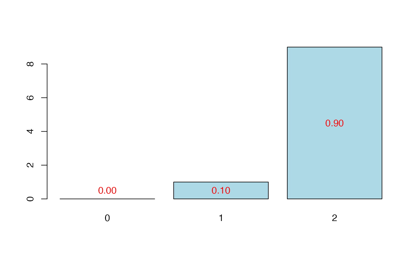
plot(cvtable(sum3))
#>
#> CV Q2Chi2 criterion:
#> 0
#> 0
#>
#> CV PreChi2 criterion:
#> 1
#> 0
 data(aze_compl)
bbb <- cv.plsRglm(y~.,data=aze_compl,nt=10,K=10,modele="pls",keepcoeffs=TRUE, verbose=FALSE)
#For Jackknife computations
kfolds2coeff(bbb)
#> [,1] [,2] [,3] [,4] [,5] [,6]
#> [1,] 0.17952318 -0.18358069 0.5161098 -0.1970097 0.3432269 0.14406722
#> [2,] 0.35486763 -0.13637388 0.3957869 -0.2173580 0.3219187 0.03170179
#> [3,] 0.33521485 -0.11313171 0.3619222 -0.2489085 0.2235826 0.14783733
#> [4,] 0.36137537 -0.13489880 0.4751676 -0.1456797 0.3143053 0.07825339
#> [5,] 0.39892318 -0.14974277 0.4912091 -0.1333353 0.2465573 0.04141418
#> [6,] 0.35575963 -0.15979357 0.4360585 -0.1439848 0.1418600 0.09004068
#> [7,] 0.36192756 -0.16936160 0.3541551 -0.1643634 0.2103803 0.17025162
#> [8,] 0.37423079 -0.11674480 0.4160774 -0.1919962 0.2852640 0.13706961
#> [9,] -0.02132443 -0.10957065 0.5659451 -0.2705819 0.3429421 0.11972351
#> [10,] 0.22012069 -0.06492909 0.5845200 -0.1663546 0.3168039 0.04866365
#> [,7] [,8] [,9] [,10] [,11]
#> [1,] 0.005055119 -0.038703832 -0.2571432 0.146789151 -0.168382704
#> [2,] -0.019036273 -0.003253334 -0.2559151 0.118744491 -0.075399509
#> [3,] -0.121191704 0.107641274 -0.1411623 0.093327808 -0.059216708
#> [4,] -0.152479468 0.023338255 -0.1098179 0.008658965 -0.141339811
#> [5,] -0.111047521 -0.023397267 -0.2485575 -0.065852638 -0.038422674
#> [6,] -0.015909361 0.007412513 -0.1291427 0.063113505 -0.057988769
#> [7,] -0.093195865 0.042269770 -0.1805481 -0.003189911 -0.125462227
#> [8,] -0.116861565 -0.002197013 -0.2515660 0.032865891 0.017641030
#> [9,] -0.012303380 -0.046829189 -0.2522609 0.041513610 -0.007180318
#> [10,] 0.060093993 0.065599396 -0.2409495 0.037350847 -0.204718238
#> [,12] [,13] [,14] [,15] [,16] [,17]
#> [1,] 0.1249068075 -0.17751959 0.10265542 0.007837119 0.10071757 0.118916503
#> [2,] -0.0022470110 -0.12354564 0.12454837 0.039703445 0.01694103 0.022199126
#> [3,] 0.0752765026 -0.04104846 0.07988420 0.066697127 0.07220045 0.009193862
#> [4,] 0.0243577425 -0.08327565 0.14772026 0.089837980 0.12111513 0.004168097
#> [5,] 0.0706978339 -0.16541495 0.15677722 0.183976063 -0.05341081 0.060792750
#> [6,] 0.0200666191 -0.06576887 0.06466309 0.117137444 0.03326864 -0.029718013
#> [7,] 0.0754839409 -0.10527587 0.12421903 0.184423100 0.04300596 -0.105705980
#> [8,] 0.0055059576 -0.09703297 0.14873490 0.080873461 0.08790355 -0.050843806
#> [9,] 0.1244068338 -0.24806077 0.10833856 0.118967892 0.06089489 0.002948510
#> [10,] -0.0002526879 -0.18986208 0.08533294 0.187802532 0.08557121 0.053980146
#> [,18] [,19] [,20] [,21] [,22] [,23]
#> [1,] 0.2350007 -0.042572440 0.11002000 -0.17439453 0.11034362 0.27575858
#> [2,] 0.2924087 0.010195821 0.06649023 -0.11157999 0.08148841 0.20909839
#> [3,] 0.1810613 0.049828840 -0.01354591 -0.22894350 0.13780002 0.19368056
#> [4,] 0.2280875 -0.007786965 -0.01794921 -0.10961352 0.13152759 0.05164439
#> [5,] 0.1814771 0.044180255 0.11897818 -0.09146756 -0.02083331 0.26713912
#> [6,] 0.2114864 -0.073119375 0.07654015 -0.18757912 0.07562632 0.16732477
#> [7,] 0.2884797 0.061275351 0.08129355 -0.06677417 0.07334575 0.11644107
#> [8,] 0.2495068 0.048902989 0.10683997 -0.06861327 0.06705986 0.15148672
#> [9,] 0.3647231 -0.021627249 0.05201960 -0.05902643 0.08953918 0.18270856
#> [10,] 0.1907015 0.064084386 0.18049238 -0.10081597 -0.07573383 0.27895839
#> [,24] [,25] [,26] [,27] [,28] [,29]
#> [1,] -0.21923953 -0.2446405 -0.3733561 0.19518539 0.2252522 -0.18334833
#> [2,] -0.19784877 -0.1763453 -0.3101657 0.20005392 0.1613447 -0.04828271
#> [3,] -0.10504568 -0.1764676 -0.2070636 0.09461131 0.2380637 -0.07371022
#> [4,] -0.15396328 -0.2432382 -0.2015450 0.21816483 0.1523498 -0.12841479
#> [5,] -0.14435273 -0.1305746 -0.3134875 0.12506679 0.1454776 -0.10287116
#> [6,] -0.08353783 -0.1654616 -0.2942352 0.23180525 0.2992130 -0.07559580
#> [7,] -0.07799205 -0.1208744 -0.3483218 0.17504792 0.1808582 -0.08645249
#> [8,] -0.14895954 -0.1674702 -0.3162844 0.23426714 0.2464161 -0.18714513
#> [9,] -0.19616815 -0.0310772 -0.2753396 0.20505455 0.1873829 -0.11823695
#> [10,] -0.15493743 -0.3530348 -0.2561731 0.15461451 0.1007065 -0.02512739
#> [,30] [,31] [,32] [,33] [,34]
#> [1,] 0.065690072 0.088159481 -0.0322657267 -0.2784938 0.042173811
#> [2,] 0.009509667 0.182200256 -0.0863661964 -0.3992084 0.043228795
#> [3,] -0.031892160 0.148228132 -0.0687252063 -0.4172826 -0.081560209
#> [4,] 0.023731318 0.126998699 -0.0359740247 -0.4201255 0.037335195
#> [5,] 0.061829943 -0.028519777 0.0004144259 -0.3579925 0.040781211
#> [6,] -0.051164051 0.115084495 0.0446461823 -0.5016755 -0.003751708
#> [7,] -0.019958880 0.177658366 -0.0183375618 -0.4407841 -0.091256937
#> [8,] 0.021704477 0.111346123 -0.0931150117 -0.4516393 -0.010121379
#> [9,] 0.054898697 0.206397884 -0.1818664097 -0.3522866 -0.029160853
#> [10,] 0.032878376 0.006803997 0.0331389178 -0.3266800 -0.038402853
bbb2 <- cv.plsRglm(y~.,data=aze_compl,nt=10,K=10,modele="pls-glm-family",
family=binomial(probit),keepcoeffs=TRUE, verbose=FALSE)
bbb2 <- cv.plsRglm(y~.,data=aze_compl,nt=10,K=10,
modele="pls-glm-logistic",keepcoeffs=TRUE, verbose=FALSE)
summary(bbb,MClassed=TRUE)
#> ____************************************************____
#>
#> Model: pls
#>
#> ____Component____ 1 ____
#> ____Component____ 2 ____
#> ____Component____ 3 ____
#> ____Component____ 4 ____
#> ____Component____ 5 ____
#> ____Component____ 6 ____
#> ____Component____ 7 ____
#> ____Component____ 8 ____
#> ____Component____ 9 ____
#> ____Component____ 10 ____
#> ____Predicting X without NA neither in X or Y____
#> ****________________________________________________****
#>
#>
#> NK: 1
#> [[1]]
#> AIC MissClassed CV_MissClassed Q2cum_Y LimQ2_Y Q2_Y
#> Nb_Comp_0 154.6179 49 NA NA NA NA
#> Nb_Comp_1 126.4083 27 49 -0.1768169 0.0975 -0.1768169
#> Nb_Comp_2 119.3375 25 48 -0.8158860 0.0975 -0.5430488
#> Nb_Comp_3 114.2313 27 49 -2.4018547 0.0975 -0.8733856
#> Nb_Comp_4 112.3463 23 50 -6.5321615 0.0975 -1.2141338
#> Nb_Comp_5 113.2362 22 50 -16.2613341 0.0975 -1.2916840
#> Nb_Comp_6 114.7620 21 50 -39.7178594 0.0975 -1.3589057
#> Nb_Comp_7 116.5264 20 50 -95.8630906 0.0975 -1.3788846
#> Nb_Comp_8 118.4601 20 51 -231.0774120 0.0975 -1.3959323
#> Nb_Comp_9 120.4452 19 51 -556.5611537 0.0975 -1.4024792
#> Nb_Comp_10 122.4395 19 51 -1338.2107374 0.0975 -1.4019083
#> PRESS_Y RSS_Y R2_Y AIC.std DoF.dof sigmahat.dof AIC.dof
#> Nb_Comp_0 NA 25.91346 NA 298.1344 1.00000 0.5015845 0.2540061
#> Nb_Comp_1 30.49540 19.38086 0.2520929 269.9248 22.55372 0.4848429 0.2883114
#> Nb_Comp_2 29.90562 17.76209 0.3145613 262.8540 27.31542 0.4781670 0.2908950
#> Nb_Comp_3 33.27524 16.58896 0.3598323 257.7478 30.52370 0.4719550 0.2902572
#> Nb_Comp_4 36.73018 15.98071 0.3833049 255.8628 34.00000 0.4744263 0.3008285
#> Nb_Comp_5 36.62273 15.81104 0.3898523 256.7527 34.00000 0.4719012 0.2976347
#> Nb_Comp_6 37.29675 15.73910 0.3926285 258.2785 34.00000 0.4708264 0.2962804
#> Nb_Comp_7 37.44150 15.70350 0.3940024 260.0429 33.71066 0.4693382 0.2937976
#> Nb_Comp_8 37.62451 15.69348 0.3943888 261.9766 34.00000 0.4701436 0.2954217
#> Nb_Comp_9 37.70326 15.69123 0.3944758 263.9617 33.87284 0.4696894 0.2945815
#> Nb_Comp_10 37.68889 15.69037 0.3945088 265.9560 34.00000 0.4700970 0.2953632
#> BIC.dof GMDL.dof DoF.naive sigmahat.naive AIC.naive BIC.naive
#> Nb_Comp_0 0.2604032 -67.17645 1 0.5015845 0.2540061 0.2604032
#> Nb_Comp_1 0.4231184 -53.56607 2 0.4358996 0.1936625 0.2033251
#> Nb_Comp_2 0.4496983 -52.42272 3 0.4193593 0.1809352 0.1943501
#> Nb_Comp_3 0.4631316 -51.93343 4 0.4072955 0.1722700 0.1891422
#> Nb_Comp_4 0.4954133 -50.37079 5 0.4017727 0.1691819 0.1897041
#> Nb_Comp_5 0.4901536 -50.65724 6 0.4016679 0.1706451 0.1952588
#> Nb_Comp_6 0.4879234 -50.78005 7 0.4028135 0.1731800 0.2020601
#> Nb_Comp_7 0.4826103 -51.05525 8 0.4044479 0.1761610 0.2094352
#> Nb_Comp_8 0.4865092 -50.85833 9 0.4064413 0.1794902 0.2172936
#> Nb_Comp_9 0.4845867 -50.95616 10 0.4085682 0.1829787 0.2254232
#> Nb_Comp_10 0.4864128 -50.86368 11 0.4107477 0.1865584 0.2337468
#> GMDL.naive
#> Nb_Comp_0 -67.17645
#> Nb_Comp_1 -79.67755
#> Nb_Comp_2 -81.93501
#> Nb_Comp_3 -83.31503
#> Nb_Comp_4 -83.23369
#> Nb_Comp_5 -81.93513
#> Nb_Comp_6 -80.42345
#> Nb_Comp_7 -78.87607
#> Nb_Comp_8 -77.31942
#> Nb_Comp_9 -75.80069
#> Nb_Comp_10 -74.33325
#>
#> attr(,"class")
#> [1] "summary.cv.plsRmodel"
summary(bbb2,MClassed=TRUE)
#> ____************************************************____
#>
#> Family: binomial
#> Link function: logit
#>
#> ____Component____ 1 ____
#> ____Component____ 2 ____
#> ____Component____ 3 ____
#> ____Component____ 4 ____
#> ____Component____ 5 ____
#> ____Component____ 6 ____
#> ____Component____ 7 ____
#> ____Component____ 8 ____
#> ____Component____ 9 ____
#> ____Component____ 10 ____
#> ____Predicting X without NA neither in X or Y____
#> ****________________________________________________****
#>
#>
#> NK: 1
#> [[1]]
#> AIC BIC MissClassed CV_MissClassed Q2Chisqcum_Y limQ2
#> Nb_Comp_0 145.8283 148.4727 49 NA NA NA
#> Nb_Comp_1 118.1398 123.4285 28 NA NA 0.0975
#> Nb_Comp_2 109.9553 117.8885 26 NA NA 0.0975
#> Nb_Comp_3 105.1591 115.7366 22 NA NA 0.0975
#> Nb_Comp_4 103.8382 117.0601 21 NA NA 0.0975
#> Nb_Comp_5 104.7338 120.6001 21 NA NA 0.0975
#> Nb_Comp_6 105.6770 124.1878 21 NA NA 0.0975
#> Nb_Comp_7 107.2828 128.4380 20 NA NA 0.0975
#> Nb_Comp_8 109.0172 132.8167 22 NA NA 0.0975
#> Nb_Comp_9 110.9354 137.3793 21 NA NA 0.0975
#> Nb_Comp_10 112.9021 141.9904 20 NA NA 0.0975
#> Q2Chisq_Y PREChi2_Pearson_Y Chi2_Pearson_Y RSS_Y R2_Y
#> Nb_Comp_0 NA NA 104.00000 25.91346 NA
#> Nb_Comp_1 NA NA 100.53823 19.32272 0.2543365
#> Nb_Comp_2 NA NA 99.17955 17.33735 0.3309519
#> Nb_Comp_3 NA NA 123.37836 15.58198 0.3986915
#> Nb_Comp_4 NA NA 114.77551 15.14046 0.4157299
#> Nb_Comp_5 NA NA 105.35382 15.08411 0.4179043
#> Nb_Comp_6 NA NA 98.87767 14.93200 0.4237744
#> Nb_Comp_7 NA NA 97.04072 14.87506 0.4259715
#> Nb_Comp_8 NA NA 98.90110 14.84925 0.4269676
#> Nb_Comp_9 NA NA 100.35563 14.84317 0.4272022
#> Nb_Comp_10 NA NA 102.85214 14.79133 0.4292027
#>
#> attr(,"class")
#> [1] "summary.cv.plsRglmmodel"
kfolds2coeff(bbb2)
#> [,1] [,2] [,3] [,4] [,5] [,6] [,7]
#> [1,] -1.965799 -1.0199331 3.648911 -1.827265 2.662801 0.8363928 -0.20691823
#> [2,] -1.830537 -0.7563970 2.471137 -1.328305 1.373733 0.2233750 -0.01177607
#> [3,] -2.407847 -2.0298046 3.945164 -1.373957 1.150147 0.5031490 -0.28988306
#> [4,] -3.203007 -2.8372141 5.033710 -2.342386 2.849491 0.5291630 -0.35109681
#> [5,] -3.921451 -2.3715250 4.589552 -2.449563 3.207610 1.0504067 -0.28974803
#> [6,] -3.282263 -1.0293596 3.976786 -1.858869 2.238536 0.1722852 -0.05050652
#> [7,] -2.812126 -0.6713289 5.375383 -1.346515 3.262103 -0.3730782 0.54959518
#> [8,] -1.927544 -1.1442212 3.731474 -3.196959 3.488297 0.9931449 -0.44058243
#> [9,] -1.531716 -0.8715758 3.034173 -1.404271 1.773505 0.6354226 0.11996263
#> [10,] -2.414664 -0.3558774 3.794280 -1.785590 1.969097 1.6414859 -0.25026263
#> [,8] [,9] [,10] [,11] [,12] [,13]
#> [1,] -0.49557050 -2.2071901 0.3144860 -0.54202797 0.89228175 -1.3974488
#> [2,] 0.08175729 -0.8963582 0.3744940 -0.82162989 0.95615239 -0.9206204
#> [3,] 0.43607504 -0.3824681 0.3625755 -1.45131465 0.84913838 -0.3492717
#> [4,] -0.58858681 -1.2308754 1.7161346 -1.43443870 0.69995889 -1.4772216
#> [5,] -0.35619065 -1.8369971 -0.5525098 -0.89540254 1.90236001 -1.0874626
#> [6,] -0.37069014 -1.1498791 -0.0109854 -0.54891131 0.37492146 -0.5548299
#> [7,] -0.30273554 -2.3051430 0.6134508 -1.03987768 0.29071503 -1.0123951
#> [8,] 0.72584141 -1.4468813 0.6799241 -1.48397492 0.74533508 -0.3907250
#> [9,] -0.92881692 -1.4740544 0.2470470 -0.78119954 0.46362094 -1.2201283
#> [10,] -0.50050095 -1.6644052 0.9803552 -0.05002341 -0.02921065 -1.8217372
#> [,14] [,15] [,16] [,17] [,18] [,19]
#> [1,] 0.4358246 0.6140765 0.4353961 1.03774234 1.831834 -0.196193746
#> [2,] 0.4477398 0.9288757 0.3006236 0.13455052 1.987615 -0.100381114
#> [3,] 0.3238327 1.3386612 -0.1676638 1.05782999 1.098517 0.615658509
#> [4,] 1.8742007 0.5617816 3.9698098 1.75700382 1.849360 -1.337655891
#> [5,] -0.1440952 1.5457708 -0.2065585 0.42532822 3.712537 0.334844801
#> [6,] 0.6290360 0.2229422 0.6668117 0.67706931 1.594161 0.001342479
#> [7,] 0.2792567 1.0277483 0.6998584 0.71725754 1.622390 0.400745609
#> [8,] 0.4989434 0.3625643 0.6576075 0.05803996 2.996122 -0.013229745
#> [9,] 0.8207341 0.8339903 0.5055199 0.60297127 1.527743 -0.430524781
#> [10,] 2.6738156 0.8785213 0.2864730 0.12896572 1.034729 0.113203504
#> [,20] [,21] [,22] [,23] [,24] [,25]
#> [1,] 0.972378415 -0.4871654 0.5628326 1.8361471 -1.28128703 -1.988099
#> [2,] 0.627611896 -0.6617926 0.7704099 1.5821050 -1.33485590 -1.477002
#> [3,] 1.174386144 -1.2668516 0.2016689 0.8706718 -0.07905719 -2.052309
#> [4,] 1.595173575 -2.4129503 1.3251517 -0.5706750 -0.93031259 -2.544465
#> [5,] 1.116156919 -1.5859034 0.1183023 1.8599384 -1.50675883 -1.298512
#> [6,] 0.303664715 -0.3820341 0.1644571 1.4632345 -1.39241213 -1.340381
#> [7,] 0.183816922 -1.4149841 -0.4554074 2.0560514 -1.35446911 -1.867863
#> [8,] -0.098670036 -1.1387885 0.4048529 1.1567518 -2.55717510 -1.480850
#> [9,] 0.739530460 -1.0162033 0.1812029 1.7540139 -0.88453664 -1.599275
#> [10,] 0.007075075 -0.9902770 0.6096433 1.2025498 -1.56825066 -1.090705
#> [,26] [,27] [,28] [,29] [,30] [,31] [,32]
#> [1,] -2.337064 1.388788 1.5932181 -0.5114985 0.7249617 1.0289371 -0.4060729
#> [2,] -1.787068 1.183226 1.3537645 -0.3917539 0.5019871 0.7369473 -0.4116624
#> [3,] -2.629235 2.833334 2.1034713 -0.2423233 -0.5243678 1.6754232 -0.3921395
#> [4,] -1.430462 0.695463 1.5404238 -0.4989249 0.4161941 1.3803824 -0.3206621
#> [5,] -2.792315 2.118639 1.5949681 -0.7218437 0.3504715 1.8499016 0.4807796
#> [6,] -1.558588 1.458914 1.4431533 -0.5113983 0.5674723 1.9399099 -0.4903038
#> [7,] -2.215763 1.773044 0.9484737 -0.6892981 0.6376707 1.1413413 0.2866099
#> [8,] -3.023586 1.985707 2.0889874 0.4568915 0.8408701 1.5481679 -0.9643611
#> [9,] -1.775669 1.827119 1.3916357 -0.3777829 0.2414968 0.9526591 -0.2185785
#> [10,] -2.488184 1.647320 2.1733116 -1.3909588 0.7063196 1.5892143 -0.4530108
#> [,33] [,34]
#> [1,] -2.785066 -0.30193814
#> [2,] -2.818961 0.16363750
#> [3,] -3.901225 -0.03908195
#> [4,] -3.593725 -0.14883634
#> [5,] -3.359821 -0.30516790
#> [6,] -2.883337 0.30333766
#> [7,] -3.519127 0.05782243
#> [8,] -4.382122 0.53328853
#> [9,] -2.264007 -0.09067303
#> [10,] -3.599580 0.15623576
kfolds2Chisqind(bbb2)
#> [[1]]
#> [[1]][[1]]
#> [1] NA NA NA NA NA NA NA NA NA NA
#>
#> [[1]][[2]]
#> [1] NA NA NA NA NA NA NA NA NA NA
#>
#> [[1]][[3]]
#> [1] NA NA NA NA NA NA NA NA NA NA
#>
#> [[1]][[4]]
#> [1] NA NA NA NA NA NA NA NA NA NA
#>
#> [[1]][[5]]
#> [1] NA NA NA NA NA NA NA NA NA NA
#>
#> [[1]][[6]]
#> [1] NA NA NA NA NA NA NA NA NA NA
#>
#> [[1]][[7]]
#> [1] NA NA NA NA NA NA NA NA NA NA
#>
#> [[1]][[8]]
#> [1] NA NA NA NA NA NA NA NA NA NA
#>
#> [[1]][[9]]
#> [1] NA NA NA NA NA NA NA NA NA NA
#>
#> [[1]][[10]]
#> [1] NA NA NA NA NA NA NA NA NA NA
#>
#>
kfolds2Chisq(bbb2)
#> [[1]]
#> [1] NA NA NA NA NA NA NA NA NA NA
#>
summary(bbb2)
#> ____************************************************____
#>
#> Family: binomial
#> Link function: logit
#>
#> ____Component____ 1 ____
#> ____Component____ 2 ____
#> ____Component____ 3 ____
#> ____Component____ 4 ____
#> ____Component____ 5 ____
#> ____Component____ 6 ____
#> ____Component____ 7 ____
#> ____Component____ 8 ____
#> ____Component____ 9 ____
#> ____Component____ 10 ____
#> ____Predicting X without NA neither in X or Y____
#> ****________________________________________________****
#>
#>
#> NK: 1
#> [[1]]
#> AIC BIC Q2Chisqcum_Y limQ2 Q2Chisq_Y PREChi2_Pearson_Y
#> Nb_Comp_0 145.8283 148.4727 NA NA NA NA
#> Nb_Comp_1 118.1398 123.4285 NA 0.0975 NA NA
#> Nb_Comp_2 109.9553 117.8885 NA 0.0975 NA NA
#> Nb_Comp_3 105.1591 115.7366 NA 0.0975 NA NA
#> Nb_Comp_4 103.8382 117.0601 NA 0.0975 NA NA
#> Nb_Comp_5 104.7338 120.6001 NA 0.0975 NA NA
#> Nb_Comp_6 105.6770 124.1878 NA 0.0975 NA NA
#> Nb_Comp_7 107.2828 128.4380 NA 0.0975 NA NA
#> Nb_Comp_8 109.0172 132.8167 NA 0.0975 NA NA
#> Nb_Comp_9 110.9354 137.3793 NA 0.0975 NA NA
#> Nb_Comp_10 112.9021 141.9904 NA 0.0975 NA NA
#> Chi2_Pearson_Y RSS_Y R2_Y
#> Nb_Comp_0 104.00000 25.91346 NA
#> Nb_Comp_1 100.53823 19.32272 0.2543365
#> Nb_Comp_2 99.17955 17.33735 0.3309519
#> Nb_Comp_3 123.37836 15.58198 0.3986915
#> Nb_Comp_4 114.77551 15.14046 0.4157299
#> Nb_Comp_5 105.35382 15.08411 0.4179043
#> Nb_Comp_6 98.87767 14.93200 0.4237744
#> Nb_Comp_7 97.04072 14.87506 0.4259715
#> Nb_Comp_8 98.90110 14.84925 0.4269676
#> Nb_Comp_9 100.35563 14.84317 0.4272022
#> Nb_Comp_10 102.85214 14.79133 0.4292027
#>
#> attr(,"class")
#> [1] "summary.cv.plsRglmmodel"
rm(list=c("bbb","bbb2"))
data(pine)
Xpine<-pine[,1:10]
ypine<-pine[,11]
bbb <- cv.plsRglm(round(x11)~.,data=pine,nt=10,modele="pls-glm-family",
family=poisson(log),K=10,keepcoeffs=TRUE,keepfolds=FALSE,verbose=FALSE)
bbb <- cv.plsRglm(round(x11)~.,data=pine,nt=10,
modele="pls-glm-poisson",K=10,keepcoeffs=TRUE,keepfolds=FALSE,verbose=FALSE)
#For Jackknife computations
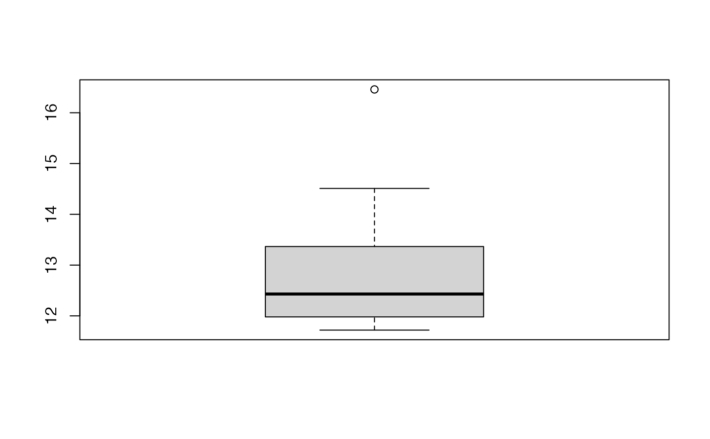
kfolds2coeff(bbb)
#> [,1] [,2] [,3] [,4] [,5] [,6]
#> [1,] 12.23228 -0.005536853 -0.06035313 0.21075559 -1.509566 0.3891260
#> [2,] 14.32616 -0.005472639 -0.07659818 0.25653307 -1.496063 0.2455091
#> [3,] 12.40342 -0.004631656 -0.10646369 0.16293855 -2.485515 0.4488413
#> [4,] 10.97834 -0.004237452 -0.05073310 0.17068724 -1.595761 0.3037007
#> [5,] 11.99869 -0.004589766 -0.07217495 0.19467679 -1.301550 0.2616567
#> [6,] 11.21735 -0.004246082 -0.07199980 0.15406592 -1.438080 0.2934104
#> [7,] 16.85425 -0.006536052 -0.09856612 0.34244991 -2.109424 0.4062731
#> [8,] 10.92865 -0.005912708 -0.03022862 -0.02194749 -1.316067 0.2801402
#> [9,] 11.28964 -0.004643210 -0.07253036 0.15351588 -1.612797 0.3242276
#> [10,] 14.59362 -0.005455122 -0.05837141 0.25584500 -1.779435 0.3188999
#> [,7] [,8] [,9] [,10] [,11]
#> [1,] -2.2221164 0.154839413 -0.0148678 -0.9159189 -0.043456849
#> [2,] -2.9221081 0.036086621 0.3780611 -1.5914109 -0.201445332
#> [3,] -2.0592645 0.663714218 0.5454282 -1.1510459 -0.627219682
#> [4,] -1.6471132 0.142996046 0.1627417 -1.3784248 -0.006574006
#> [5,] -1.8966704 -0.224268493 0.1396611 -1.3784609 0.164126510
#> [6,] -1.6236813 0.002402134 0.1512606 -0.9878680 -0.307230536
#> [7,] -4.3402151 0.359188340 0.3560064 -1.1404673 -0.372509115
#> [8,] 0.4838324 -0.522774677 0.1006362 -1.0965444 -0.011750707
#> [9,] -1.5812611 0.141304409 0.1891793 -1.0272417 -0.132808486
#> [10,] -2.9669311 0.479145437 0.2613261 -1.1668214 -0.921124035
boxplot(kfolds2coeff(bbb)[,1])
data(aze_compl)
bbb <- cv.plsRglm(y~.,data=aze_compl,nt=10,K=10,modele="pls",keepcoeffs=TRUE, verbose=FALSE)
#For Jackknife computations
kfolds2coeff(bbb)
#> [,1] [,2] [,3] [,4] [,5] [,6]
#> [1,] 0.17952318 -0.18358069 0.5161098 -0.1970097 0.3432269 0.14406722
#> [2,] 0.35486763 -0.13637388 0.3957869 -0.2173580 0.3219187 0.03170179
#> [3,] 0.33521485 -0.11313171 0.3619222 -0.2489085 0.2235826 0.14783733
#> [4,] 0.36137537 -0.13489880 0.4751676 -0.1456797 0.3143053 0.07825339
#> [5,] 0.39892318 -0.14974277 0.4912091 -0.1333353 0.2465573 0.04141418
#> [6,] 0.35575963 -0.15979357 0.4360585 -0.1439848 0.1418600 0.09004068
#> [7,] 0.36192756 -0.16936160 0.3541551 -0.1643634 0.2103803 0.17025162
#> [8,] 0.37423079 -0.11674480 0.4160774 -0.1919962 0.2852640 0.13706961
#> [9,] -0.02132443 -0.10957065 0.5659451 -0.2705819 0.3429421 0.11972351
#> [10,] 0.22012069 -0.06492909 0.5845200 -0.1663546 0.3168039 0.04866365
#> [,7] [,8] [,9] [,10] [,11]
#> [1,] 0.005055119 -0.038703832 -0.2571432 0.146789151 -0.168382704
#> [2,] -0.019036273 -0.003253334 -0.2559151 0.118744491 -0.075399509
#> [3,] -0.121191704 0.107641274 -0.1411623 0.093327808 -0.059216708
#> [4,] -0.152479468 0.023338255 -0.1098179 0.008658965 -0.141339811
#> [5,] -0.111047521 -0.023397267 -0.2485575 -0.065852638 -0.038422674
#> [6,] -0.015909361 0.007412513 -0.1291427 0.063113505 -0.057988769
#> [7,] -0.093195865 0.042269770 -0.1805481 -0.003189911 -0.125462227
#> [8,] -0.116861565 -0.002197013 -0.2515660 0.032865891 0.017641030
#> [9,] -0.012303380 -0.046829189 -0.2522609 0.041513610 -0.007180318
#> [10,] 0.060093993 0.065599396 -0.2409495 0.037350847 -0.204718238
#> [,12] [,13] [,14] [,15] [,16] [,17]
#> [1,] 0.1249068075 -0.17751959 0.10265542 0.007837119 0.10071757 0.118916503
#> [2,] -0.0022470110 -0.12354564 0.12454837 0.039703445 0.01694103 0.022199126
#> [3,] 0.0752765026 -0.04104846 0.07988420 0.066697127 0.07220045 0.009193862
#> [4,] 0.0243577425 -0.08327565 0.14772026 0.089837980 0.12111513 0.004168097
#> [5,] 0.0706978339 -0.16541495 0.15677722 0.183976063 -0.05341081 0.060792750
#> [6,] 0.0200666191 -0.06576887 0.06466309 0.117137444 0.03326864 -0.029718013
#> [7,] 0.0754839409 -0.10527587 0.12421903 0.184423100 0.04300596 -0.105705980
#> [8,] 0.0055059576 -0.09703297 0.14873490 0.080873461 0.08790355 -0.050843806
#> [9,] 0.1244068338 -0.24806077 0.10833856 0.118967892 0.06089489 0.002948510
#> [10,] -0.0002526879 -0.18986208 0.08533294 0.187802532 0.08557121 0.053980146
#> [,18] [,19] [,20] [,21] [,22] [,23]
#> [1,] 0.2350007 -0.042572440 0.11002000 -0.17439453 0.11034362 0.27575858
#> [2,] 0.2924087 0.010195821 0.06649023 -0.11157999 0.08148841 0.20909839
#> [3,] 0.1810613 0.049828840 -0.01354591 -0.22894350 0.13780002 0.19368056
#> [4,] 0.2280875 -0.007786965 -0.01794921 -0.10961352 0.13152759 0.05164439
#> [5,] 0.1814771 0.044180255 0.11897818 -0.09146756 -0.02083331 0.26713912
#> [6,] 0.2114864 -0.073119375 0.07654015 -0.18757912 0.07562632 0.16732477
#> [7,] 0.2884797 0.061275351 0.08129355 -0.06677417 0.07334575 0.11644107
#> [8,] 0.2495068 0.048902989 0.10683997 -0.06861327 0.06705986 0.15148672
#> [9,] 0.3647231 -0.021627249 0.05201960 -0.05902643 0.08953918 0.18270856
#> [10,] 0.1907015 0.064084386 0.18049238 -0.10081597 -0.07573383 0.27895839
#> [,24] [,25] [,26] [,27] [,28] [,29]
#> [1,] -0.21923953 -0.2446405 -0.3733561 0.19518539 0.2252522 -0.18334833
#> [2,] -0.19784877 -0.1763453 -0.3101657 0.20005392 0.1613447 -0.04828271
#> [3,] -0.10504568 -0.1764676 -0.2070636 0.09461131 0.2380637 -0.07371022
#> [4,] -0.15396328 -0.2432382 -0.2015450 0.21816483 0.1523498 -0.12841479
#> [5,] -0.14435273 -0.1305746 -0.3134875 0.12506679 0.1454776 -0.10287116
#> [6,] -0.08353783 -0.1654616 -0.2942352 0.23180525 0.2992130 -0.07559580
#> [7,] -0.07799205 -0.1208744 -0.3483218 0.17504792 0.1808582 -0.08645249
#> [8,] -0.14895954 -0.1674702 -0.3162844 0.23426714 0.2464161 -0.18714513
#> [9,] -0.19616815 -0.0310772 -0.2753396 0.20505455 0.1873829 -0.11823695
#> [10,] -0.15493743 -0.3530348 -0.2561731 0.15461451 0.1007065 -0.02512739
#> [,30] [,31] [,32] [,33] [,34]
#> [1,] 0.065690072 0.088159481 -0.0322657267 -0.2784938 0.042173811
#> [2,] 0.009509667 0.182200256 -0.0863661964 -0.3992084 0.043228795
#> [3,] -0.031892160 0.148228132 -0.0687252063 -0.4172826 -0.081560209
#> [4,] 0.023731318 0.126998699 -0.0359740247 -0.4201255 0.037335195
#> [5,] 0.061829943 -0.028519777 0.0004144259 -0.3579925 0.040781211
#> [6,] -0.051164051 0.115084495 0.0446461823 -0.5016755 -0.003751708
#> [7,] -0.019958880 0.177658366 -0.0183375618 -0.4407841 -0.091256937
#> [8,] 0.021704477 0.111346123 -0.0931150117 -0.4516393 -0.010121379
#> [9,] 0.054898697 0.206397884 -0.1818664097 -0.3522866 -0.029160853
#> [10,] 0.032878376 0.006803997 0.0331389178 -0.3266800 -0.038402853
bbb2 <- cv.plsRglm(y~.,data=aze_compl,nt=10,K=10,modele="pls-glm-family",
family=binomial(probit),keepcoeffs=TRUE, verbose=FALSE)
bbb2 <- cv.plsRglm(y~.,data=aze_compl,nt=10,K=10,
modele="pls-glm-logistic",keepcoeffs=TRUE, verbose=FALSE)
summary(bbb,MClassed=TRUE)
#> ____************************************************____
#>
#> Model: pls
#>
#> ____Component____ 1 ____
#> ____Component____ 2 ____
#> ____Component____ 3 ____
#> ____Component____ 4 ____
#> ____Component____ 5 ____
#> ____Component____ 6 ____
#> ____Component____ 7 ____
#> ____Component____ 8 ____
#> ____Component____ 9 ____
#> ____Component____ 10 ____
#> ____Predicting X without NA neither in X or Y____
#> ****________________________________________________****
#>
#>
#> NK: 1
#> [[1]]
#> AIC MissClassed CV_MissClassed Q2cum_Y LimQ2_Y Q2_Y
#> Nb_Comp_0 154.6179 49 NA NA NA NA
#> Nb_Comp_1 126.4083 27 49 -0.1768169 0.0975 -0.1768169
#> Nb_Comp_2 119.3375 25 48 -0.8158860 0.0975 -0.5430488
#> Nb_Comp_3 114.2313 27 49 -2.4018547 0.0975 -0.8733856
#> Nb_Comp_4 112.3463 23 50 -6.5321615 0.0975 -1.2141338
#> Nb_Comp_5 113.2362 22 50 -16.2613341 0.0975 -1.2916840
#> Nb_Comp_6 114.7620 21 50 -39.7178594 0.0975 -1.3589057
#> Nb_Comp_7 116.5264 20 50 -95.8630906 0.0975 -1.3788846
#> Nb_Comp_8 118.4601 20 51 -231.0774120 0.0975 -1.3959323
#> Nb_Comp_9 120.4452 19 51 -556.5611537 0.0975 -1.4024792
#> Nb_Comp_10 122.4395 19 51 -1338.2107374 0.0975 -1.4019083
#> PRESS_Y RSS_Y R2_Y AIC.std DoF.dof sigmahat.dof AIC.dof
#> Nb_Comp_0 NA 25.91346 NA 298.1344 1.00000 0.5015845 0.2540061
#> Nb_Comp_1 30.49540 19.38086 0.2520929 269.9248 22.55372 0.4848429 0.2883114
#> Nb_Comp_2 29.90562 17.76209 0.3145613 262.8540 27.31542 0.4781670 0.2908950
#> Nb_Comp_3 33.27524 16.58896 0.3598323 257.7478 30.52370 0.4719550 0.2902572
#> Nb_Comp_4 36.73018 15.98071 0.3833049 255.8628 34.00000 0.4744263 0.3008285
#> Nb_Comp_5 36.62273 15.81104 0.3898523 256.7527 34.00000 0.4719012 0.2976347
#> Nb_Comp_6 37.29675 15.73910 0.3926285 258.2785 34.00000 0.4708264 0.2962804
#> Nb_Comp_7 37.44150 15.70350 0.3940024 260.0429 33.71066 0.4693382 0.2937976
#> Nb_Comp_8 37.62451 15.69348 0.3943888 261.9766 34.00000 0.4701436 0.2954217
#> Nb_Comp_9 37.70326 15.69123 0.3944758 263.9617 33.87284 0.4696894 0.2945815
#> Nb_Comp_10 37.68889 15.69037 0.3945088 265.9560 34.00000 0.4700970 0.2953632
#> BIC.dof GMDL.dof DoF.naive sigmahat.naive AIC.naive BIC.naive
#> Nb_Comp_0 0.2604032 -67.17645 1 0.5015845 0.2540061 0.2604032
#> Nb_Comp_1 0.4231184 -53.56607 2 0.4358996 0.1936625 0.2033251
#> Nb_Comp_2 0.4496983 -52.42272 3 0.4193593 0.1809352 0.1943501
#> Nb_Comp_3 0.4631316 -51.93343 4 0.4072955 0.1722700 0.1891422
#> Nb_Comp_4 0.4954133 -50.37079 5 0.4017727 0.1691819 0.1897041
#> Nb_Comp_5 0.4901536 -50.65724 6 0.4016679 0.1706451 0.1952588
#> Nb_Comp_6 0.4879234 -50.78005 7 0.4028135 0.1731800 0.2020601
#> Nb_Comp_7 0.4826103 -51.05525 8 0.4044479 0.1761610 0.2094352
#> Nb_Comp_8 0.4865092 -50.85833 9 0.4064413 0.1794902 0.2172936
#> Nb_Comp_9 0.4845867 -50.95616 10 0.4085682 0.1829787 0.2254232
#> Nb_Comp_10 0.4864128 -50.86368 11 0.4107477 0.1865584 0.2337468
#> GMDL.naive
#> Nb_Comp_0 -67.17645
#> Nb_Comp_1 -79.67755
#> Nb_Comp_2 -81.93501
#> Nb_Comp_3 -83.31503
#> Nb_Comp_4 -83.23369
#> Nb_Comp_5 -81.93513
#> Nb_Comp_6 -80.42345
#> Nb_Comp_7 -78.87607
#> Nb_Comp_8 -77.31942
#> Nb_Comp_9 -75.80069
#> Nb_Comp_10 -74.33325
#>
#> attr(,"class")
#> [1] "summary.cv.plsRmodel"
summary(bbb2,MClassed=TRUE)
#> ____************************************************____
#>
#> Family: binomial
#> Link function: logit
#>
#> ____Component____ 1 ____
#> ____Component____ 2 ____
#> ____Component____ 3 ____
#> ____Component____ 4 ____
#> ____Component____ 5 ____
#> ____Component____ 6 ____
#> ____Component____ 7 ____
#> ____Component____ 8 ____
#> ____Component____ 9 ____
#> ____Component____ 10 ____
#> ____Predicting X without NA neither in X or Y____
#> ****________________________________________________****
#>
#>
#> NK: 1
#> [[1]]
#> AIC BIC MissClassed CV_MissClassed Q2Chisqcum_Y limQ2
#> Nb_Comp_0 145.8283 148.4727 49 NA NA NA
#> Nb_Comp_1 118.1398 123.4285 28 NA NA 0.0975
#> Nb_Comp_2 109.9553 117.8885 26 NA NA 0.0975
#> Nb_Comp_3 105.1591 115.7366 22 NA NA 0.0975
#> Nb_Comp_4 103.8382 117.0601 21 NA NA 0.0975
#> Nb_Comp_5 104.7338 120.6001 21 NA NA 0.0975
#> Nb_Comp_6 105.6770 124.1878 21 NA NA 0.0975
#> Nb_Comp_7 107.2828 128.4380 20 NA NA 0.0975
#> Nb_Comp_8 109.0172 132.8167 22 NA NA 0.0975
#> Nb_Comp_9 110.9354 137.3793 21 NA NA 0.0975
#> Nb_Comp_10 112.9021 141.9904 20 NA NA 0.0975
#> Q2Chisq_Y PREChi2_Pearson_Y Chi2_Pearson_Y RSS_Y R2_Y
#> Nb_Comp_0 NA NA 104.00000 25.91346 NA
#> Nb_Comp_1 NA NA 100.53823 19.32272 0.2543365
#> Nb_Comp_2 NA NA 99.17955 17.33735 0.3309519
#> Nb_Comp_3 NA NA 123.37836 15.58198 0.3986915
#> Nb_Comp_4 NA NA 114.77551 15.14046 0.4157299
#> Nb_Comp_5 NA NA 105.35382 15.08411 0.4179043
#> Nb_Comp_6 NA NA 98.87767 14.93200 0.4237744
#> Nb_Comp_7 NA NA 97.04072 14.87506 0.4259715
#> Nb_Comp_8 NA NA 98.90110 14.84925 0.4269676
#> Nb_Comp_9 NA NA 100.35563 14.84317 0.4272022
#> Nb_Comp_10 NA NA 102.85214 14.79133 0.4292027
#>
#> attr(,"class")
#> [1] "summary.cv.plsRglmmodel"
kfolds2coeff(bbb2)
#> [,1] [,2] [,3] [,4] [,5] [,6] [,7]
#> [1,] -1.965799 -1.0199331 3.648911 -1.827265 2.662801 0.8363928 -0.20691823
#> [2,] -1.830537 -0.7563970 2.471137 -1.328305 1.373733 0.2233750 -0.01177607
#> [3,] -2.407847 -2.0298046 3.945164 -1.373957 1.150147 0.5031490 -0.28988306
#> [4,] -3.203007 -2.8372141 5.033710 -2.342386 2.849491 0.5291630 -0.35109681
#> [5,] -3.921451 -2.3715250 4.589552 -2.449563 3.207610 1.0504067 -0.28974803
#> [6,] -3.282263 -1.0293596 3.976786 -1.858869 2.238536 0.1722852 -0.05050652
#> [7,] -2.812126 -0.6713289 5.375383 -1.346515 3.262103 -0.3730782 0.54959518
#> [8,] -1.927544 -1.1442212 3.731474 -3.196959 3.488297 0.9931449 -0.44058243
#> [9,] -1.531716 -0.8715758 3.034173 -1.404271 1.773505 0.6354226 0.11996263
#> [10,] -2.414664 -0.3558774 3.794280 -1.785590 1.969097 1.6414859 -0.25026263
#> [,8] [,9] [,10] [,11] [,12] [,13]
#> [1,] -0.49557050 -2.2071901 0.3144860 -0.54202797 0.89228175 -1.3974488
#> [2,] 0.08175729 -0.8963582 0.3744940 -0.82162989 0.95615239 -0.9206204
#> [3,] 0.43607504 -0.3824681 0.3625755 -1.45131465 0.84913838 -0.3492717
#> [4,] -0.58858681 -1.2308754 1.7161346 -1.43443870 0.69995889 -1.4772216
#> [5,] -0.35619065 -1.8369971 -0.5525098 -0.89540254 1.90236001 -1.0874626
#> [6,] -0.37069014 -1.1498791 -0.0109854 -0.54891131 0.37492146 -0.5548299
#> [7,] -0.30273554 -2.3051430 0.6134508 -1.03987768 0.29071503 -1.0123951
#> [8,] 0.72584141 -1.4468813 0.6799241 -1.48397492 0.74533508 -0.3907250
#> [9,] -0.92881692 -1.4740544 0.2470470 -0.78119954 0.46362094 -1.2201283
#> [10,] -0.50050095 -1.6644052 0.9803552 -0.05002341 -0.02921065 -1.8217372
#> [,14] [,15] [,16] [,17] [,18] [,19]
#> [1,] 0.4358246 0.6140765 0.4353961 1.03774234 1.831834 -0.196193746
#> [2,] 0.4477398 0.9288757 0.3006236 0.13455052 1.987615 -0.100381114
#> [3,] 0.3238327 1.3386612 -0.1676638 1.05782999 1.098517 0.615658509
#> [4,] 1.8742007 0.5617816 3.9698098 1.75700382 1.849360 -1.337655891
#> [5,] -0.1440952 1.5457708 -0.2065585 0.42532822 3.712537 0.334844801
#> [6,] 0.6290360 0.2229422 0.6668117 0.67706931 1.594161 0.001342479
#> [7,] 0.2792567 1.0277483 0.6998584 0.71725754 1.622390 0.400745609
#> [8,] 0.4989434 0.3625643 0.6576075 0.05803996 2.996122 -0.013229745
#> [9,] 0.8207341 0.8339903 0.5055199 0.60297127 1.527743 -0.430524781
#> [10,] 2.6738156 0.8785213 0.2864730 0.12896572 1.034729 0.113203504
#> [,20] [,21] [,22] [,23] [,24] [,25]
#> [1,] 0.972378415 -0.4871654 0.5628326 1.8361471 -1.28128703 -1.988099
#> [2,] 0.627611896 -0.6617926 0.7704099 1.5821050 -1.33485590 -1.477002
#> [3,] 1.174386144 -1.2668516 0.2016689 0.8706718 -0.07905719 -2.052309
#> [4,] 1.595173575 -2.4129503 1.3251517 -0.5706750 -0.93031259 -2.544465
#> [5,] 1.116156919 -1.5859034 0.1183023 1.8599384 -1.50675883 -1.298512
#> [6,] 0.303664715 -0.3820341 0.1644571 1.4632345 -1.39241213 -1.340381
#> [7,] 0.183816922 -1.4149841 -0.4554074 2.0560514 -1.35446911 -1.867863
#> [8,] -0.098670036 -1.1387885 0.4048529 1.1567518 -2.55717510 -1.480850
#> [9,] 0.739530460 -1.0162033 0.1812029 1.7540139 -0.88453664 -1.599275
#> [10,] 0.007075075 -0.9902770 0.6096433 1.2025498 -1.56825066 -1.090705
#> [,26] [,27] [,28] [,29] [,30] [,31] [,32]
#> [1,] -2.337064 1.388788 1.5932181 -0.5114985 0.7249617 1.0289371 -0.4060729
#> [2,] -1.787068 1.183226 1.3537645 -0.3917539 0.5019871 0.7369473 -0.4116624
#> [3,] -2.629235 2.833334 2.1034713 -0.2423233 -0.5243678 1.6754232 -0.3921395
#> [4,] -1.430462 0.695463 1.5404238 -0.4989249 0.4161941 1.3803824 -0.3206621
#> [5,] -2.792315 2.118639 1.5949681 -0.7218437 0.3504715 1.8499016 0.4807796
#> [6,] -1.558588 1.458914 1.4431533 -0.5113983 0.5674723 1.9399099 -0.4903038
#> [7,] -2.215763 1.773044 0.9484737 -0.6892981 0.6376707 1.1413413 0.2866099
#> [8,] -3.023586 1.985707 2.0889874 0.4568915 0.8408701 1.5481679 -0.9643611
#> [9,] -1.775669 1.827119 1.3916357 -0.3777829 0.2414968 0.9526591 -0.2185785
#> [10,] -2.488184 1.647320 2.1733116 -1.3909588 0.7063196 1.5892143 -0.4530108
#> [,33] [,34]
#> [1,] -2.785066 -0.30193814
#> [2,] -2.818961 0.16363750
#> [3,] -3.901225 -0.03908195
#> [4,] -3.593725 -0.14883634
#> [5,] -3.359821 -0.30516790
#> [6,] -2.883337 0.30333766
#> [7,] -3.519127 0.05782243
#> [8,] -4.382122 0.53328853
#> [9,] -2.264007 -0.09067303
#> [10,] -3.599580 0.15623576
kfolds2Chisqind(bbb2)
#> [[1]]
#> [[1]][[1]]
#> [1] NA NA NA NA NA NA NA NA NA NA
#>
#> [[1]][[2]]
#> [1] NA NA NA NA NA NA NA NA NA NA
#>
#> [[1]][[3]]
#> [1] NA NA NA NA NA NA NA NA NA NA
#>
#> [[1]][[4]]
#> [1] NA NA NA NA NA NA NA NA NA NA
#>
#> [[1]][[5]]
#> [1] NA NA NA NA NA NA NA NA NA NA
#>
#> [[1]][[6]]
#> [1] NA NA NA NA NA NA NA NA NA NA
#>
#> [[1]][[7]]
#> [1] NA NA NA NA NA NA NA NA NA NA
#>
#> [[1]][[8]]
#> [1] NA NA NA NA NA NA NA NA NA NA
#>
#> [[1]][[9]]
#> [1] NA NA NA NA NA NA NA NA NA NA
#>
#> [[1]][[10]]
#> [1] NA NA NA NA NA NA NA NA NA NA
#>
#>
kfolds2Chisq(bbb2)
#> [[1]]
#> [1] NA NA NA NA NA NA NA NA NA NA
#>
summary(bbb2)
#> ____************************************************____
#>
#> Family: binomial
#> Link function: logit
#>
#> ____Component____ 1 ____
#> ____Component____ 2 ____
#> ____Component____ 3 ____
#> ____Component____ 4 ____
#> ____Component____ 5 ____
#> ____Component____ 6 ____
#> ____Component____ 7 ____
#> ____Component____ 8 ____
#> ____Component____ 9 ____
#> ____Component____ 10 ____
#> ____Predicting X without NA neither in X or Y____
#> ****________________________________________________****
#>
#>
#> NK: 1
#> [[1]]
#> AIC BIC Q2Chisqcum_Y limQ2 Q2Chisq_Y PREChi2_Pearson_Y
#> Nb_Comp_0 145.8283 148.4727 NA NA NA NA
#> Nb_Comp_1 118.1398 123.4285 NA 0.0975 NA NA
#> Nb_Comp_2 109.9553 117.8885 NA 0.0975 NA NA
#> Nb_Comp_3 105.1591 115.7366 NA 0.0975 NA NA
#> Nb_Comp_4 103.8382 117.0601 NA 0.0975 NA NA
#> Nb_Comp_5 104.7338 120.6001 NA 0.0975 NA NA
#> Nb_Comp_6 105.6770 124.1878 NA 0.0975 NA NA
#> Nb_Comp_7 107.2828 128.4380 NA 0.0975 NA NA
#> Nb_Comp_8 109.0172 132.8167 NA 0.0975 NA NA
#> Nb_Comp_9 110.9354 137.3793 NA 0.0975 NA NA
#> Nb_Comp_10 112.9021 141.9904 NA 0.0975 NA NA
#> Chi2_Pearson_Y RSS_Y R2_Y
#> Nb_Comp_0 104.00000 25.91346 NA
#> Nb_Comp_1 100.53823 19.32272 0.2543365
#> Nb_Comp_2 99.17955 17.33735 0.3309519
#> Nb_Comp_3 123.37836 15.58198 0.3986915
#> Nb_Comp_4 114.77551 15.14046 0.4157299
#> Nb_Comp_5 105.35382 15.08411 0.4179043
#> Nb_Comp_6 98.87767 14.93200 0.4237744
#> Nb_Comp_7 97.04072 14.87506 0.4259715
#> Nb_Comp_8 98.90110 14.84925 0.4269676
#> Nb_Comp_9 100.35563 14.84317 0.4272022
#> Nb_Comp_10 102.85214 14.79133 0.4292027
#>
#> attr(,"class")
#> [1] "summary.cv.plsRglmmodel"
rm(list=c("bbb","bbb2"))
data(pine)
Xpine<-pine[,1:10]
ypine<-pine[,11]
bbb <- cv.plsRglm(round(x11)~.,data=pine,nt=10,modele="pls-glm-family",
family=poisson(log),K=10,keepcoeffs=TRUE,keepfolds=FALSE,verbose=FALSE)
bbb <- cv.plsRglm(round(x11)~.,data=pine,nt=10,
modele="pls-glm-poisson",K=10,keepcoeffs=TRUE,keepfolds=FALSE,verbose=FALSE)
#For Jackknife computations
kfolds2coeff(bbb)
#> [,1] [,2] [,3] [,4] [,5] [,6]
#> [1,] 12.23228 -0.005536853 -0.06035313 0.21075559 -1.509566 0.3891260
#> [2,] 14.32616 -0.005472639 -0.07659818 0.25653307 -1.496063 0.2455091
#> [3,] 12.40342 -0.004631656 -0.10646369 0.16293855 -2.485515 0.4488413
#> [4,] 10.97834 -0.004237452 -0.05073310 0.17068724 -1.595761 0.3037007
#> [5,] 11.99869 -0.004589766 -0.07217495 0.19467679 -1.301550 0.2616567
#> [6,] 11.21735 -0.004246082 -0.07199980 0.15406592 -1.438080 0.2934104
#> [7,] 16.85425 -0.006536052 -0.09856612 0.34244991 -2.109424 0.4062731
#> [8,] 10.92865 -0.005912708 -0.03022862 -0.02194749 -1.316067 0.2801402
#> [9,] 11.28964 -0.004643210 -0.07253036 0.15351588 -1.612797 0.3242276
#> [10,] 14.59362 -0.005455122 -0.05837141 0.25584500 -1.779435 0.3188999
#> [,7] [,8] [,9] [,10] [,11]
#> [1,] -2.2221164 0.154839413 -0.0148678 -0.9159189 -0.043456849
#> [2,] -2.9221081 0.036086621 0.3780611 -1.5914109 -0.201445332
#> [3,] -2.0592645 0.663714218 0.5454282 -1.1510459 -0.627219682
#> [4,] -1.6471132 0.142996046 0.1627417 -1.3784248 -0.006574006
#> [5,] -1.8966704 -0.224268493 0.1396611 -1.3784609 0.164126510
#> [6,] -1.6236813 0.002402134 0.1512606 -0.9878680 -0.307230536
#> [7,] -4.3402151 0.359188340 0.3560064 -1.1404673 -0.372509115
#> [8,] 0.4838324 -0.522774677 0.1006362 -1.0965444 -0.011750707
#> [9,] -1.5812611 0.141304409 0.1891793 -1.0272417 -0.132808486
#> [10,] -2.9669311 0.479145437 0.2613261 -1.1668214 -0.921124035
boxplot(kfolds2coeff(bbb)[,1])
 kfolds2Chisqind(bbb)
#> [[1]]
#> [[1]][[1]]
#> [1] NA NA NA NA NA NA NA NA NA NA
#>
#> [[1]][[2]]
#> [1] NA NA NA NA NA NA NA NA NA NA
#>
#> [[1]][[3]]
#> [1] NA NA NA NA NA NA NA NA NA NA
#>
#> [[1]][[4]]
#> [1] NA NA NA NA NA NA NA NA NA NA
#>
#> [[1]][[5]]
#> [1] NA NA NA NA NA NA NA NA NA NA
#>
#> [[1]][[6]]
#> [1] NA NA NA NA NA NA NA NA NA NA
#>
#> [[1]][[7]]
#> [1] NA NA NA NA NA NA NA NA NA NA
#>
#> [[1]][[8]]
#> [1] NA NA NA NA NA NA NA NA NA NA
#>
#> [[1]][[9]]
#> [1] NA NA NA NA NA NA NA NA NA NA
#>
#> [[1]][[10]]
#> [1] NA NA NA NA NA NA NA NA NA NA
#>
#>
kfolds2Chisq(bbb)
#> [[1]]
#> [1] NA NA NA NA NA NA NA NA NA NA
#>
summary(bbb)
#> ____************************************************____
#>
#> Family: poisson
#> Link function: log
#>
#> ____Component____ 1 ____
#> ____Component____ 2 ____
#> ____Component____ 3 ____
#> ____Component____ 4 ____
#> ____Component____ 5 ____
#> ____Component____ 6 ____
#> ____Component____ 7 ____
#> ____Component____ 8 ____
#> ____Component____ 9 ____
#> ____Component____ 10 ____
#> ____Predicting X without NA neither in X or Y____
#> ****________________________________________________****
#>
#>
#> NK: 1
#> [[1]]
#> AIC BIC Q2Chisqcum_Y limQ2 Q2Chisq_Y PREChi2_Pearson_Y
#> Nb_Comp_0 76.61170 78.10821 NA NA NA NA
#> Nb_Comp_1 65.70029 68.69331 NA 0.0975 NA NA
#> Nb_Comp_2 62.49440 66.98392 NA 0.0975 NA NA
#> Nb_Comp_3 62.47987 68.46590 NA 0.0975 NA NA
#> Nb_Comp_4 64.21704 71.69958 NA 0.0975 NA NA
#> Nb_Comp_5 65.81654 74.79559 NA 0.0975 NA NA
#> Nb_Comp_6 66.48888 76.96443 NA 0.0975 NA NA
#> Nb_Comp_7 68.40234 80.37440 NA 0.0975 NA NA
#> Nb_Comp_8 70.39399 83.86256 NA 0.0975 NA NA
#> Nb_Comp_9 72.37642 87.34149 NA 0.0975 NA NA
#> Nb_Comp_10 74.37612 90.83770 NA 0.0975 NA NA
#> Chi2_Pearson_Y RSS_Y R2_Y
#> Nb_Comp_0 33.75000 24.545455 NA
#> Nb_Comp_1 23.85891 12.599337 0.4866937
#> Nb_Comp_2 17.29992 9.056074 0.6310488
#> Nb_Comp_3 15.50937 8.232069 0.6646194
#> Nb_Comp_4 15.23934 8.125808 0.6689485
#> Nb_Comp_5 15.26275 7.862134 0.6796909
#> Nb_Comp_6 17.74629 6.203270 0.7472742
#> Nb_Comp_7 18.04460 5.879880 0.7604493
#> Nb_Comp_8 18.17881 5.827065 0.7626011
#> Nb_Comp_9 18.34925 5.837300 0.7621841
#> Nb_Comp_10 18.39332 5.832437 0.7623822
#>
#> attr(,"class")
#> [1] "summary.cv.plsRglmmodel"
PLS_lm(ypine,Xpine,10,typeVC="standard")$InfCrit
#> ____************************************************____
#> ____TypeVC____ standard ____
#> ____Component____ 1 ____
#> ____Component____ 2 ____
#> ____Component____ 3 ____
#> ____Component____ 4 ____
#> ____Component____ 5 ____
#> ____Component____ 6 ____
#> ____Component____ 7 ____
#> ____Component____ 8 ____
#> ____Component____ 9 ____
#> ____Component____ 10 ____
#> ____Predicting X without NA neither in X nor in Y____
#> ****________________________________________________****
#>
#> AIC Q2cum_Y LimQ2_Y Q2_Y PRESS_Y RSS_Y
#> Nb_Comp_0 82.41888 NA NA NA NA 20.800152
#> Nb_Comp_1 63.61896 0.38248575 0.0975 0.38248575 12.844390 11.074659
#> Nb_Comp_2 58.47638 0.34836456 0.0975 -0.05525570 11.686597 8.919303
#> Nb_Comp_3 56.55421 0.23688359 0.0975 -0.17107874 10.445206 7.919786
#> Nb_Comp_4 54.35053 0.06999681 0.0975 -0.21869112 9.651773 6.972542
#> Nb_Comp_5 55.99834 -0.07691053 0.0975 -0.15796434 8.073955 6.898523
#> Nb_Comp_6 57.69592 -0.19968885 0.0975 -0.11400977 7.685022 6.835594
#> Nb_Comp_7 59.37953 -0.27722139 0.0975 -0.06462721 7.277359 6.770369
#> Nb_Comp_8 61.21213 -0.30602578 0.0975 -0.02255238 6.923057 6.736112
#> Nb_Comp_9 63.18426 -0.39920228 0.0975 -0.07134354 7.216690 6.730426
#> Nb_Comp_10 65.15982 -0.43743644 0.0975 -0.02732569 6.914340 6.725443
#> R2_Y R2_residY RSS_residY PRESS_residY Q2_residY LimQ2
#> Nb_Comp_0 NA NA 32.00000 NA NA NA
#> Nb_Comp_1 0.4675684 0.4675684 17.03781 19.76046 0.38248575 0.0975
#> Nb_Comp_2 0.5711905 0.5711905 13.72190 17.97925 -0.05525570 0.0975
#> Nb_Comp_3 0.6192438 0.6192438 12.18420 16.06943 -0.17107874 0.0975
#> Nb_Comp_4 0.6647841 0.6647841 10.72691 14.84877 -0.21869112 0.0975
#> Nb_Comp_5 0.6683426 0.6683426 10.61304 12.42138 -0.15796434 0.0975
#> Nb_Comp_6 0.6713681 0.6713681 10.51622 11.82303 -0.11400977 0.0975
#> Nb_Comp_7 0.6745039 0.6745039 10.41588 11.19586 -0.06462721 0.0975
#> Nb_Comp_8 0.6761508 0.6761508 10.36317 10.65078 -0.02255238 0.0975
#> Nb_Comp_9 0.6764242 0.6764242 10.35443 11.10252 -0.07134354 0.0975
#> Nb_Comp_10 0.6766638 0.6766638 10.34676 10.63737 -0.02732569 0.0975
#> Q2cum_residY AIC.std DoF.dof sigmahat.dof AIC.dof BIC.dof
#> Nb_Comp_0 NA 96.63448 1.000000 0.8062287 0.6697018 0.6991787
#> Nb_Comp_1 0.38248575 77.83455 3.176360 0.5994089 0.4047616 0.4565153
#> Nb_Comp_2 0.34836456 72.69198 7.133559 0.5761829 0.4138120 0.5212090
#> Nb_Comp_3 0.23688359 70.76981 8.778329 0.5603634 0.4070516 0.5320535
#> Nb_Comp_4 0.06999681 68.56612 8.427874 0.5221703 0.3505594 0.4547689
#> Nb_Comp_5 -0.07691053 70.21393 9.308247 0.5285695 0.3666578 0.4845912
#> Nb_Comp_6 -0.19968885 71.91152 9.291931 0.5259794 0.3629363 0.4795121
#> Nb_Comp_7 -0.27722139 73.59512 9.756305 0.5284535 0.3702885 0.4938445
#> Nb_Comp_8 -0.30602578 75.42772 10.363948 0.5338475 0.3831339 0.5170783
#> Nb_Comp_9 -0.39920228 77.39986 10.732145 0.5378276 0.3920956 0.5328746
#> Nb_Comp_10 -0.43743644 79.37542 11.000000 0.5407500 0.3987417 0.5446065
#> GMDL.dof DoF.naive sigmahat.naive AIC.naive BIC.naive GMDL.naive
#> Nb_Comp_0 -3.605128 1 0.8062287 0.6697018 0.6991787 -3.605128
#> Nb_Comp_1 -9.875081 2 0.5977015 0.3788984 0.4112998 -11.451340
#> Nb_Comp_2 -6.985517 3 0.5452615 0.3243383 0.3647862 -12.822703
#> Nb_Comp_3 -6.260610 4 0.5225859 0.3061986 0.3557368 -12.756838
#> Nb_Comp_4 -8.152986 5 0.4990184 0.2867496 0.3432131 -12.811575
#> Nb_Comp_5 -7.111583 6 0.5054709 0.3019556 0.3714754 -11.329638
#> Nb_Comp_6 -7.233043 7 0.5127450 0.3186757 0.4021333 -9.918688
#> Nb_Comp_7 -6.742195 8 0.5203986 0.3364668 0.4347156 -8.592770
#> Nb_Comp_8 -6.038372 9 0.5297842 0.3572181 0.4717708 -7.287834
#> Nb_Comp_9 -5.600238 10 0.5409503 0.3813021 0.5140048 -6.008747
#> Nb_Comp_10 -5.288422 11 0.5529032 0.4076026 0.5600977 -4.799453
data(pineNAX21)
bbb2 <- cv.plsRglm(round(x11)~.,data=pineNAX21,nt=10,
modele="pls-glm-family",family=poisson(log),K=10,keepcoeffs=TRUE,keepfolds=FALSE,verbose=FALSE)
bbb2 <- cv.plsRglm(round(x11)~.,data=pineNAX21,nt=10,
modele="pls-glm-poisson",K=10,keepcoeffs=TRUE,keepfolds=FALSE,verbose=FALSE)
#For Jackknife computations
kfolds2coeff(bbb2)
#> [,1] [,2] [,3] [,4] [,5] [,6]
#> [1,] 11.51811 -0.005952386 -0.04705644 0.01579405 -1.519639 0.3274029
#> [2,] 13.48966 -0.004981385 -0.06984414 0.19631381 -1.560965 0.3040376
#> [3,] 12.63692 -0.004543425 -0.05466002 0.15527180 -1.371838 0.2951140
#> [4,] 12.81233 -0.005251442 -0.05779519 0.19878499 -1.341721 0.3182705
#> [5,] 13.30235 -0.004022254 -0.09036926 0.20118035 -2.168910 0.4199286
#> [6,] 15.62810 -0.006164254 -0.08473175 0.22820188 -1.902573 0.3330847
#> [7,] 13.61742 -0.005004306 -0.06550345 0.19769215 -1.506993 0.2906218
#> [8,] 13.82062 -0.005346061 -0.06939079 0.25433075 -1.570217 0.2798791
#> [9,] 19.74373 -0.007589103 -0.10421749 0.37990696 -2.120497 0.4017688
#> [10,] 14.84834 -0.004928453 -0.04972723 0.24531299 -1.503833 0.2712783
#> [,7] [,8] [,9] [,10] [,11]
#> [1,] -0.2014834 0.10523208 0.06110290 -0.4074067 -0.12976644
#> [2,] -2.2805101 0.04360632 0.24608496 -1.0725974 -0.29707532
#> [3,] -1.2419615 -0.34704147 0.02554851 -1.3843230 0.11912524
#> [4,] -1.9245434 0.01273538 0.08933275 -1.5051381 0.26169495
#> [5,] -2.2112053 0.18672331 0.30611669 -1.3219579 -0.32977787
#> [6,] -2.6356030 0.42081192 0.41712124 -1.3295615 -0.48652744
#> [7,] -2.0755348 -0.06300028 0.22280792 -1.3888067 -0.16197199
#> [8,] -2.7872614 0.05704597 0.28563651 -1.5290880 -0.09594567
#> [9,] -5.0683254 0.81985345 0.45414536 -1.0032677 -0.83199603
#> [10,] -2.6971167 0.03780900 0.20135091 -1.4205660 -0.61724236
boxplot(kfolds2coeff(bbb2)[,1])
kfolds2Chisqind(bbb)
#> [[1]]
#> [[1]][[1]]
#> [1] NA NA NA NA NA NA NA NA NA NA
#>
#> [[1]][[2]]
#> [1] NA NA NA NA NA NA NA NA NA NA
#>
#> [[1]][[3]]
#> [1] NA NA NA NA NA NA NA NA NA NA
#>
#> [[1]][[4]]
#> [1] NA NA NA NA NA NA NA NA NA NA
#>
#> [[1]][[5]]
#> [1] NA NA NA NA NA NA NA NA NA NA
#>
#> [[1]][[6]]
#> [1] NA NA NA NA NA NA NA NA NA NA
#>
#> [[1]][[7]]
#> [1] NA NA NA NA NA NA NA NA NA NA
#>
#> [[1]][[8]]
#> [1] NA NA NA NA NA NA NA NA NA NA
#>
#> [[1]][[9]]
#> [1] NA NA NA NA NA NA NA NA NA NA
#>
#> [[1]][[10]]
#> [1] NA NA NA NA NA NA NA NA NA NA
#>
#>
kfolds2Chisq(bbb)
#> [[1]]
#> [1] NA NA NA NA NA NA NA NA NA NA
#>
summary(bbb)
#> ____************************************************____
#>
#> Family: poisson
#> Link function: log
#>
#> ____Component____ 1 ____
#> ____Component____ 2 ____
#> ____Component____ 3 ____
#> ____Component____ 4 ____
#> ____Component____ 5 ____
#> ____Component____ 6 ____
#> ____Component____ 7 ____
#> ____Component____ 8 ____
#> ____Component____ 9 ____
#> ____Component____ 10 ____
#> ____Predicting X without NA neither in X or Y____
#> ****________________________________________________****
#>
#>
#> NK: 1
#> [[1]]
#> AIC BIC Q2Chisqcum_Y limQ2 Q2Chisq_Y PREChi2_Pearson_Y
#> Nb_Comp_0 76.61170 78.10821 NA NA NA NA
#> Nb_Comp_1 65.70029 68.69331 NA 0.0975 NA NA
#> Nb_Comp_2 62.49440 66.98392 NA 0.0975 NA NA
#> Nb_Comp_3 62.47987 68.46590 NA 0.0975 NA NA
#> Nb_Comp_4 64.21704 71.69958 NA 0.0975 NA NA
#> Nb_Comp_5 65.81654 74.79559 NA 0.0975 NA NA
#> Nb_Comp_6 66.48888 76.96443 NA 0.0975 NA NA
#> Nb_Comp_7 68.40234 80.37440 NA 0.0975 NA NA
#> Nb_Comp_8 70.39399 83.86256 NA 0.0975 NA NA
#> Nb_Comp_9 72.37642 87.34149 NA 0.0975 NA NA
#> Nb_Comp_10 74.37612 90.83770 NA 0.0975 NA NA
#> Chi2_Pearson_Y RSS_Y R2_Y
#> Nb_Comp_0 33.75000 24.545455 NA
#> Nb_Comp_1 23.85891 12.599337 0.4866937
#> Nb_Comp_2 17.29992 9.056074 0.6310488
#> Nb_Comp_3 15.50937 8.232069 0.6646194
#> Nb_Comp_4 15.23934 8.125808 0.6689485
#> Nb_Comp_5 15.26275 7.862134 0.6796909
#> Nb_Comp_6 17.74629 6.203270 0.7472742
#> Nb_Comp_7 18.04460 5.879880 0.7604493
#> Nb_Comp_8 18.17881 5.827065 0.7626011
#> Nb_Comp_9 18.34925 5.837300 0.7621841
#> Nb_Comp_10 18.39332 5.832437 0.7623822
#>
#> attr(,"class")
#> [1] "summary.cv.plsRglmmodel"
PLS_lm(ypine,Xpine,10,typeVC="standard")$InfCrit
#> ____************************************************____
#> ____TypeVC____ standard ____
#> ____Component____ 1 ____
#> ____Component____ 2 ____
#> ____Component____ 3 ____
#> ____Component____ 4 ____
#> ____Component____ 5 ____
#> ____Component____ 6 ____
#> ____Component____ 7 ____
#> ____Component____ 8 ____
#> ____Component____ 9 ____
#> ____Component____ 10 ____
#> ____Predicting X without NA neither in X nor in Y____
#> ****________________________________________________****
#>
#> AIC Q2cum_Y LimQ2_Y Q2_Y PRESS_Y RSS_Y
#> Nb_Comp_0 82.41888 NA NA NA NA 20.800152
#> Nb_Comp_1 63.61896 0.38248575 0.0975 0.38248575 12.844390 11.074659
#> Nb_Comp_2 58.47638 0.34836456 0.0975 -0.05525570 11.686597 8.919303
#> Nb_Comp_3 56.55421 0.23688359 0.0975 -0.17107874 10.445206 7.919786
#> Nb_Comp_4 54.35053 0.06999681 0.0975 -0.21869112 9.651773 6.972542
#> Nb_Comp_5 55.99834 -0.07691053 0.0975 -0.15796434 8.073955 6.898523
#> Nb_Comp_6 57.69592 -0.19968885 0.0975 -0.11400977 7.685022 6.835594
#> Nb_Comp_7 59.37953 -0.27722139 0.0975 -0.06462721 7.277359 6.770369
#> Nb_Comp_8 61.21213 -0.30602578 0.0975 -0.02255238 6.923057 6.736112
#> Nb_Comp_9 63.18426 -0.39920228 0.0975 -0.07134354 7.216690 6.730426
#> Nb_Comp_10 65.15982 -0.43743644 0.0975 -0.02732569 6.914340 6.725443
#> R2_Y R2_residY RSS_residY PRESS_residY Q2_residY LimQ2
#> Nb_Comp_0 NA NA 32.00000 NA NA NA
#> Nb_Comp_1 0.4675684 0.4675684 17.03781 19.76046 0.38248575 0.0975
#> Nb_Comp_2 0.5711905 0.5711905 13.72190 17.97925 -0.05525570 0.0975
#> Nb_Comp_3 0.6192438 0.6192438 12.18420 16.06943 -0.17107874 0.0975
#> Nb_Comp_4 0.6647841 0.6647841 10.72691 14.84877 -0.21869112 0.0975
#> Nb_Comp_5 0.6683426 0.6683426 10.61304 12.42138 -0.15796434 0.0975
#> Nb_Comp_6 0.6713681 0.6713681 10.51622 11.82303 -0.11400977 0.0975
#> Nb_Comp_7 0.6745039 0.6745039 10.41588 11.19586 -0.06462721 0.0975
#> Nb_Comp_8 0.6761508 0.6761508 10.36317 10.65078 -0.02255238 0.0975
#> Nb_Comp_9 0.6764242 0.6764242 10.35443 11.10252 -0.07134354 0.0975
#> Nb_Comp_10 0.6766638 0.6766638 10.34676 10.63737 -0.02732569 0.0975
#> Q2cum_residY AIC.std DoF.dof sigmahat.dof AIC.dof BIC.dof
#> Nb_Comp_0 NA 96.63448 1.000000 0.8062287 0.6697018 0.6991787
#> Nb_Comp_1 0.38248575 77.83455 3.176360 0.5994089 0.4047616 0.4565153
#> Nb_Comp_2 0.34836456 72.69198 7.133559 0.5761829 0.4138120 0.5212090
#> Nb_Comp_3 0.23688359 70.76981 8.778329 0.5603634 0.4070516 0.5320535
#> Nb_Comp_4 0.06999681 68.56612 8.427874 0.5221703 0.3505594 0.4547689
#> Nb_Comp_5 -0.07691053 70.21393 9.308247 0.5285695 0.3666578 0.4845912
#> Nb_Comp_6 -0.19968885 71.91152 9.291931 0.5259794 0.3629363 0.4795121
#> Nb_Comp_7 -0.27722139 73.59512 9.756305 0.5284535 0.3702885 0.4938445
#> Nb_Comp_8 -0.30602578 75.42772 10.363948 0.5338475 0.3831339 0.5170783
#> Nb_Comp_9 -0.39920228 77.39986 10.732145 0.5378276 0.3920956 0.5328746
#> Nb_Comp_10 -0.43743644 79.37542 11.000000 0.5407500 0.3987417 0.5446065
#> GMDL.dof DoF.naive sigmahat.naive AIC.naive BIC.naive GMDL.naive
#> Nb_Comp_0 -3.605128 1 0.8062287 0.6697018 0.6991787 -3.605128
#> Nb_Comp_1 -9.875081 2 0.5977015 0.3788984 0.4112998 -11.451340
#> Nb_Comp_2 -6.985517 3 0.5452615 0.3243383 0.3647862 -12.822703
#> Nb_Comp_3 -6.260610 4 0.5225859 0.3061986 0.3557368 -12.756838
#> Nb_Comp_4 -8.152986 5 0.4990184 0.2867496 0.3432131 -12.811575
#> Nb_Comp_5 -7.111583 6 0.5054709 0.3019556 0.3714754 -11.329638
#> Nb_Comp_6 -7.233043 7 0.5127450 0.3186757 0.4021333 -9.918688
#> Nb_Comp_7 -6.742195 8 0.5203986 0.3364668 0.4347156 -8.592770
#> Nb_Comp_8 -6.038372 9 0.5297842 0.3572181 0.4717708 -7.287834
#> Nb_Comp_9 -5.600238 10 0.5409503 0.3813021 0.5140048 -6.008747
#> Nb_Comp_10 -5.288422 11 0.5529032 0.4076026 0.5600977 -4.799453
data(pineNAX21)
bbb2 <- cv.plsRglm(round(x11)~.,data=pineNAX21,nt=10,
modele="pls-glm-family",family=poisson(log),K=10,keepcoeffs=TRUE,keepfolds=FALSE,verbose=FALSE)
bbb2 <- cv.plsRglm(round(x11)~.,data=pineNAX21,nt=10,
modele="pls-glm-poisson",K=10,keepcoeffs=TRUE,keepfolds=FALSE,verbose=FALSE)
#For Jackknife computations
kfolds2coeff(bbb2)
#> [,1] [,2] [,3] [,4] [,5] [,6]
#> [1,] 11.51811 -0.005952386 -0.04705644 0.01579405 -1.519639 0.3274029
#> [2,] 13.48966 -0.004981385 -0.06984414 0.19631381 -1.560965 0.3040376
#> [3,] 12.63692 -0.004543425 -0.05466002 0.15527180 -1.371838 0.2951140
#> [4,] 12.81233 -0.005251442 -0.05779519 0.19878499 -1.341721 0.3182705
#> [5,] 13.30235 -0.004022254 -0.09036926 0.20118035 -2.168910 0.4199286
#> [6,] 15.62810 -0.006164254 -0.08473175 0.22820188 -1.902573 0.3330847
#> [7,] 13.61742 -0.005004306 -0.06550345 0.19769215 -1.506993 0.2906218
#> [8,] 13.82062 -0.005346061 -0.06939079 0.25433075 -1.570217 0.2798791
#> [9,] 19.74373 -0.007589103 -0.10421749 0.37990696 -2.120497 0.4017688
#> [10,] 14.84834 -0.004928453 -0.04972723 0.24531299 -1.503833 0.2712783
#> [,7] [,8] [,9] [,10] [,11]
#> [1,] -0.2014834 0.10523208 0.06110290 -0.4074067 -0.12976644
#> [2,] -2.2805101 0.04360632 0.24608496 -1.0725974 -0.29707532
#> [3,] -1.2419615 -0.34704147 0.02554851 -1.3843230 0.11912524
#> [4,] -1.9245434 0.01273538 0.08933275 -1.5051381 0.26169495
#> [5,] -2.2112053 0.18672331 0.30611669 -1.3219579 -0.32977787
#> [6,] -2.6356030 0.42081192 0.41712124 -1.3295615 -0.48652744
#> [7,] -2.0755348 -0.06300028 0.22280792 -1.3888067 -0.16197199
#> [8,] -2.7872614 0.05704597 0.28563651 -1.5290880 -0.09594567
#> [9,] -5.0683254 0.81985345 0.45414536 -1.0032677 -0.83199603
#> [10,] -2.6971167 0.03780900 0.20135091 -1.4205660 -0.61724236
boxplot(kfolds2coeff(bbb2)[,1])
 kfolds2Chisqind(bbb2)
#> [[1]]
#> [[1]][[1]]
#> [1] NA NA NA NA NA NA NA NA NA
#>
#> [[1]][[2]]
#> [1] NA NA NA NA NA NA NA NA NA
#>
#> [[1]][[3]]
#> [1] NA NA NA NA NA NA NA NA NA
#>
#> [[1]][[4]]
#> [1] NA NA NA NA NA NA NA NA NA
#>
#> [[1]][[5]]
#> [1] NA NA NA NA NA NA NA NA NA
#>
#> [[1]][[6]]
#> [1] NA NA NA NA NA NA NA NA NA
#>
#> [[1]][[7]]
#> [1] NA NA NA NA NA NA NA NA NA
#>
#> [[1]][[8]]
#> [1] NA NA NA NA NA NA NA NA NA
#>
#> [[1]][[9]]
#> [1] NA NA NA NA NA NA NA NA NA
#>
#> [[1]][[10]]
#> [1] NA NA NA NA NA NA NA NA NA
#>
#>
kfolds2Chisq(bbb2)
#> [[1]]
#> [1] NA NA NA NA NA NA NA NA NA
#>
summary(bbb2)
#> ____************************************************____
#> Only naive DoF can be used with missing data
#>
#> Family: poisson
#> Link function: log
#>
#> ____There are some NAs in X but not in Y____
#> ____Component____ 1 ____
#> ____Component____ 2 ____
#> ____Component____ 3 ____
#> ____Component____ 4 ____
#> ____Component____ 5 ____
#> ____Component____ 6 ____
#> ____Component____ 7 ____
#> ____Component____ 8 ____
#> ____Component____ 9 ____
#> ____Predicting X with NA in X and not in Y____
#> ****________________________________________________****
#>
#>
#> NK: 1
#> [[1]]
#> AIC BIC Q2Chisqcum_Y limQ2 Q2Chisq_Y PREChi2_Pearson_Y
#> Nb_Comp_0 76.61170 78.10821 NA NA NA NA
#> Nb_Comp_1 65.74449 68.73751 NA 0.0975 NA NA
#> Nb_Comp_2 62.35674 66.84626 NA 0.0975 NA NA
#> Nb_Comp_3 62.39804 68.38407 NA 0.0975 NA NA
#> Nb_Comp_4 64.08113 71.56366 NA 0.0975 NA NA
#> Nb_Comp_5 65.63784 74.61689 NA 0.0975 NA NA
#> Nb_Comp_6 67.18468 77.66024 NA 0.0975 NA NA
#> Nb_Comp_7 68.61004 80.58210 NA 0.0975 NA NA
#> Nb_Comp_8 70.54487 84.01344 NA 0.0975 NA NA
#> Nb_Comp_9 72.37296 87.33803 NA 0.0975 NA NA
#> Chi2_Pearson_Y RSS_Y R2_Y
#> Nb_Comp_0 33.75000 24.545455 NA
#> Nb_Comp_1 23.89105 12.654950 0.4844280
#> Nb_Comp_2 17.31172 8.871122 0.6385839
#> Nb_Comp_3 15.51670 8.203709 0.6657748
#> Nb_Comp_4 15.31216 7.959332 0.6757309
#> Nb_Comp_5 15.51159 7.724832 0.6852846
#> Nb_Comp_6 16.30549 6.814620 0.7223673
#> Nb_Comp_7 17.52007 6.284737 0.7439552
#> Nb_Comp_8 17.75766 6.160827 0.7490034
#> Nb_Comp_9 18.30206 5.831059 0.7624383
#>
#> attr(,"class")
#> [1] "summary.cv.plsRglmmodel"
data(XpineNAX21)
PLS_lm(ypine,XpineNAX21,10,typeVC="standard")$InfCrit
#> ____************************************************____
#> Only naive DoF can be used with missing data
#> ____There are some NAs in X but not in Y____
#> ____TypeVC____ standard ____
#> ____Component____ 1 ____
#> ____Component____ 2 ____
#> ____Component____ 3 ____
#> ____Component____ 4 ____
#> ____Component____ 5 ____
#> ____Component____ 6 ____
#> ____Component____ 7 ____
#> ____Component____ 8 ____
#> ____Component____ 9 ____
#> Warning : reciprocal condition number of t(cbind(res$pp,temppp)[XXNA[1,],,drop=FALSE])%*%cbind(res$pp,temppp)[XXNA[1,],,drop=FALSE] < 10^{-12}
#> Warning only 9 components could thus be extracted
#> ____Predicting X with NA in X and not in Y____
#> ****________________________________________________****
#>
#> AIC Q2cum_Y LimQ2_Y Q2_Y PRESS_Y RSS_Y
#> Nb_Comp_0 82.41888 NA NA NA NA 20.800152
#> Nb_Comp_1 63.69250 0.35639805 0.0975 0.35639805 13.387018 11.099368
#> Nb_Comp_2 58.35228 0.28395028 0.0975 -0.11256611 12.348781 8.885823
#> Nb_Comp_3 56.36553 0.07664889 0.0975 -0.28950699 11.458331 7.874634
#> Nb_Comp_4 54.02416 -0.70355579 0.0975 -0.84497074 14.528469 6.903925
#> Nb_Comp_5 55.80450 -0.94905654 0.0975 -0.14411078 7.898855 6.858120
#> Nb_Comp_6 57.45753 -1.27568315 0.0975 -0.16758190 8.007417 6.786392
#> Nb_Comp_7 58.73951 -1.63309014 0.0975 -0.15705481 7.852227 6.640327
#> Nb_Comp_8 60.61227 -1.67907859 0.0975 -0.01746558 6.756304 6.614773
#> Nb_Comp_9 62.25948 -2.15165796 0.0975 -0.17639623 7.781594 6.544432
#> R2_Y R2_residY RSS_residY PRESS_residY Q2_residY LimQ2
#> Nb_Comp_0 NA NA 32.00000 NA NA NA
#> Nb_Comp_1 0.4663804 0.4663804 17.07583 20.59526 0.35639805 0.0975
#> Nb_Comp_2 0.5728001 0.5728001 13.67040 18.99799 -0.11256611 0.0975
#> Nb_Comp_3 0.6214146 0.6214146 12.11473 17.62807 -0.28950699 0.0975
#> Nb_Comp_4 0.6680830 0.6680830 10.62135 22.35133 -0.84497074 0.0975
#> Nb_Comp_5 0.6702851 0.6702851 10.55088 12.15200 -0.14411078 0.0975
#> Nb_Comp_6 0.6737336 0.6737336 10.44053 12.31901 -0.16758190 0.0975
#> Nb_Comp_7 0.6807558 0.6807558 10.21581 12.08026 -0.15705481 0.0975
#> Nb_Comp_8 0.6819844 0.6819844 10.17650 10.39424 -0.01746558 0.0975
#> Nb_Comp_9 0.6853661 0.6853661 10.06828 11.97160 -0.17639623 0.0975
#> Q2cum_residY AIC.std DoF.dof sigmahat.dof AIC.dof BIC.dof GMDL.dof
#> Nb_Comp_0 NA 96.63448 NA NA NA NA NA
#> Nb_Comp_1 0.35639805 77.90810 NA NA NA NA NA
#> Nb_Comp_2 0.28395028 72.56787 NA NA NA NA NA
#> Nb_Comp_3 0.07664889 70.58113 NA NA NA NA NA
#> Nb_Comp_4 -0.70355579 68.23976 NA NA NA NA NA
#> Nb_Comp_5 -0.94905654 70.02009 NA NA NA NA NA
#> Nb_Comp_6 -1.27568315 71.67313 NA NA NA NA NA
#> Nb_Comp_7 -1.63309014 72.95511 NA NA NA NA NA
#> Nb_Comp_8 -1.67907859 74.82787 NA NA NA NA NA
#> Nb_Comp_9 -2.15165796 76.47507 NA NA NA NA NA
#> DoF.naive sigmahat.naive AIC.naive BIC.naive GMDL.naive
#> Nb_Comp_0 1 0.8062287 0.6697018 0.6991787 -3.605128
#> Nb_Comp_1 2 0.5983679 0.3797438 0.4122175 -11.413749
#> Nb_Comp_2 3 0.5442372 0.3231208 0.3634169 -12.847656
#> Nb_Comp_3 4 0.5210941 0.3044529 0.3537087 -12.776843
#> Nb_Comp_4 5 0.4965569 0.2839276 0.3398355 -12.891035
#> Nb_Comp_5 6 0.5039885 0.3001871 0.3692997 -11.349498
#> Nb_Comp_6 7 0.5108963 0.3163819 0.3992388 -9.922119
#> Nb_Comp_7 8 0.5153766 0.3300041 0.4263658 -8.696873
#> Nb_Comp_8 9 0.5249910 0.3507834 0.4632727 -7.337679
#> Nb_Comp_9 10 0.5334234 0.3707649 0.4998004 -6.033403
rm(list=c("Xpine","XpineNAX21","ypine","bbb","bbb2"))
#> Warning: object 'XpineNAX21' not found
data(pine)
Xpine<-pine[,1:10]
ypine<-pine[,11]
bbb <- cv.plsRglm(x11~.,data=pine,nt=10,modele="pls-glm-family",
family=Gamma,K=10,keepcoeffs=TRUE,keepfolds=FALSE,verbose=FALSE)
#> Warning: NaNs produced
bbb <- cv.plsRglm(x11~.,data=pine,nt=10,modele="pls-glm-Gamma",
K=10,keepcoeffs=TRUE,keepfolds=FALSE,verbose=FALSE)
#For Jackknife computations
kfolds2coeff(bbb)
#> [,1] [,2] [,3] [,4] [,5] [,6]
#> [1,] -12.538587 0.006081631 0.051485268 -0.17200406 1.9564449 -0.4121492
#> [2,] -12.361937 0.009237988 0.039134946 -0.32515811 2.0576931 -0.3290479
#> [3,] -9.057436 0.004677511 0.007988804 -0.07922100 0.9813196 -0.2186069
#> [4,] -10.586646 0.005689529 0.032376860 -0.09035462 1.9699193 -0.3928204
#> [5,] -10.927667 0.004506554 0.030789213 -0.21565214 1.3977266 -0.2934423
#> [6,] -11.501775 0.005522298 0.051836980 -0.13536601 1.5245202 -0.3109914
#> [7,] -16.494083 0.005806689 0.095088328 -0.32343382 3.6142443 -0.6056931
#> [8,] -9.210819 0.007641321 -0.008129801 0.13439933 1.6843999 -0.3819648
#> [9,] -13.596107 0.007307016 0.062945208 -0.25963003 1.7436597 -0.3738348
#> [10,] -11.656738 0.005533928 0.040602824 -0.16403631 1.7953572 -0.3669673
#> [,7] [,8] [,9] [,10] [,11]
#> [1,] 2.3545656 -0.4281201 -0.197686771 0.7935866 0.7913407
#> [2,] 3.3769636 -4.2565134 -0.553253701 2.5194587 0.8576111
#> [3,] 0.9108687 0.2556929 0.004448834 1.0393063 0.2458766
#> [4,] 1.3923929 -0.7220402 -0.193888178 0.4000389 1.0641619
#> [5,] 2.6197499 -0.1320216 -0.081918997 1.0256996 0.5635740
#> [6,] 1.3504613 -0.1576628 -0.130366130 1.2050842 0.4686387
#> [7,] 4.3052478 -0.6259748 -0.740700803 1.5778828 0.8433978
#> [8,] -1.4808742 -0.1824521 -0.090878056 0.7290671 0.4302643
#> [9,] 4.2000986 -0.9848552 -0.134796298 -0.5740824 0.8225901
#> [10,] 2.2218202 -0.3694189 -0.189664822 0.8733890 0.7222851
boxplot(kfolds2coeff(bbb)[,1])
kfolds2Chisqind(bbb2)
#> [[1]]
#> [[1]][[1]]
#> [1] NA NA NA NA NA NA NA NA NA
#>
#> [[1]][[2]]
#> [1] NA NA NA NA NA NA NA NA NA
#>
#> [[1]][[3]]
#> [1] NA NA NA NA NA NA NA NA NA
#>
#> [[1]][[4]]
#> [1] NA NA NA NA NA NA NA NA NA
#>
#> [[1]][[5]]
#> [1] NA NA NA NA NA NA NA NA NA
#>
#> [[1]][[6]]
#> [1] NA NA NA NA NA NA NA NA NA
#>
#> [[1]][[7]]
#> [1] NA NA NA NA NA NA NA NA NA
#>
#> [[1]][[8]]
#> [1] NA NA NA NA NA NA NA NA NA
#>
#> [[1]][[9]]
#> [1] NA NA NA NA NA NA NA NA NA
#>
#> [[1]][[10]]
#> [1] NA NA NA NA NA NA NA NA NA
#>
#>
kfolds2Chisq(bbb2)
#> [[1]]
#> [1] NA NA NA NA NA NA NA NA NA
#>
summary(bbb2)
#> ____************************************************____
#> Only naive DoF can be used with missing data
#>
#> Family: poisson
#> Link function: log
#>
#> ____There are some NAs in X but not in Y____
#> ____Component____ 1 ____
#> ____Component____ 2 ____
#> ____Component____ 3 ____
#> ____Component____ 4 ____
#> ____Component____ 5 ____
#> ____Component____ 6 ____
#> ____Component____ 7 ____
#> ____Component____ 8 ____
#> ____Component____ 9 ____
#> ____Predicting X with NA in X and not in Y____
#> ****________________________________________________****
#>
#>
#> NK: 1
#> [[1]]
#> AIC BIC Q2Chisqcum_Y limQ2 Q2Chisq_Y PREChi2_Pearson_Y
#> Nb_Comp_0 76.61170 78.10821 NA NA NA NA
#> Nb_Comp_1 65.74449 68.73751 NA 0.0975 NA NA
#> Nb_Comp_2 62.35674 66.84626 NA 0.0975 NA NA
#> Nb_Comp_3 62.39804 68.38407 NA 0.0975 NA NA
#> Nb_Comp_4 64.08113 71.56366 NA 0.0975 NA NA
#> Nb_Comp_5 65.63784 74.61689 NA 0.0975 NA NA
#> Nb_Comp_6 67.18468 77.66024 NA 0.0975 NA NA
#> Nb_Comp_7 68.61004 80.58210 NA 0.0975 NA NA
#> Nb_Comp_8 70.54487 84.01344 NA 0.0975 NA NA
#> Nb_Comp_9 72.37296 87.33803 NA 0.0975 NA NA
#> Chi2_Pearson_Y RSS_Y R2_Y
#> Nb_Comp_0 33.75000 24.545455 NA
#> Nb_Comp_1 23.89105 12.654950 0.4844280
#> Nb_Comp_2 17.31172 8.871122 0.6385839
#> Nb_Comp_3 15.51670 8.203709 0.6657748
#> Nb_Comp_4 15.31216 7.959332 0.6757309
#> Nb_Comp_5 15.51159 7.724832 0.6852846
#> Nb_Comp_6 16.30549 6.814620 0.7223673
#> Nb_Comp_7 17.52007 6.284737 0.7439552
#> Nb_Comp_8 17.75766 6.160827 0.7490034
#> Nb_Comp_9 18.30206 5.831059 0.7624383
#>
#> attr(,"class")
#> [1] "summary.cv.plsRglmmodel"
data(XpineNAX21)
PLS_lm(ypine,XpineNAX21,10,typeVC="standard")$InfCrit
#> ____************************************************____
#> Only naive DoF can be used with missing data
#> ____There are some NAs in X but not in Y____
#> ____TypeVC____ standard ____
#> ____Component____ 1 ____
#> ____Component____ 2 ____
#> ____Component____ 3 ____
#> ____Component____ 4 ____
#> ____Component____ 5 ____
#> ____Component____ 6 ____
#> ____Component____ 7 ____
#> ____Component____ 8 ____
#> ____Component____ 9 ____
#> Warning : reciprocal condition number of t(cbind(res$pp,temppp)[XXNA[1,],,drop=FALSE])%*%cbind(res$pp,temppp)[XXNA[1,],,drop=FALSE] < 10^{-12}
#> Warning only 9 components could thus be extracted
#> ____Predicting X with NA in X and not in Y____
#> ****________________________________________________****
#>
#> AIC Q2cum_Y LimQ2_Y Q2_Y PRESS_Y RSS_Y
#> Nb_Comp_0 82.41888 NA NA NA NA 20.800152
#> Nb_Comp_1 63.69250 0.35639805 0.0975 0.35639805 13.387018 11.099368
#> Nb_Comp_2 58.35228 0.28395028 0.0975 -0.11256611 12.348781 8.885823
#> Nb_Comp_3 56.36553 0.07664889 0.0975 -0.28950699 11.458331 7.874634
#> Nb_Comp_4 54.02416 -0.70355579 0.0975 -0.84497074 14.528469 6.903925
#> Nb_Comp_5 55.80450 -0.94905654 0.0975 -0.14411078 7.898855 6.858120
#> Nb_Comp_6 57.45753 -1.27568315 0.0975 -0.16758190 8.007417 6.786392
#> Nb_Comp_7 58.73951 -1.63309014 0.0975 -0.15705481 7.852227 6.640327
#> Nb_Comp_8 60.61227 -1.67907859 0.0975 -0.01746558 6.756304 6.614773
#> Nb_Comp_9 62.25948 -2.15165796 0.0975 -0.17639623 7.781594 6.544432
#> R2_Y R2_residY RSS_residY PRESS_residY Q2_residY LimQ2
#> Nb_Comp_0 NA NA 32.00000 NA NA NA
#> Nb_Comp_1 0.4663804 0.4663804 17.07583 20.59526 0.35639805 0.0975
#> Nb_Comp_2 0.5728001 0.5728001 13.67040 18.99799 -0.11256611 0.0975
#> Nb_Comp_3 0.6214146 0.6214146 12.11473 17.62807 -0.28950699 0.0975
#> Nb_Comp_4 0.6680830 0.6680830 10.62135 22.35133 -0.84497074 0.0975
#> Nb_Comp_5 0.6702851 0.6702851 10.55088 12.15200 -0.14411078 0.0975
#> Nb_Comp_6 0.6737336 0.6737336 10.44053 12.31901 -0.16758190 0.0975
#> Nb_Comp_7 0.6807558 0.6807558 10.21581 12.08026 -0.15705481 0.0975
#> Nb_Comp_8 0.6819844 0.6819844 10.17650 10.39424 -0.01746558 0.0975
#> Nb_Comp_9 0.6853661 0.6853661 10.06828 11.97160 -0.17639623 0.0975
#> Q2cum_residY AIC.std DoF.dof sigmahat.dof AIC.dof BIC.dof GMDL.dof
#> Nb_Comp_0 NA 96.63448 NA NA NA NA NA
#> Nb_Comp_1 0.35639805 77.90810 NA NA NA NA NA
#> Nb_Comp_2 0.28395028 72.56787 NA NA NA NA NA
#> Nb_Comp_3 0.07664889 70.58113 NA NA NA NA NA
#> Nb_Comp_4 -0.70355579 68.23976 NA NA NA NA NA
#> Nb_Comp_5 -0.94905654 70.02009 NA NA NA NA NA
#> Nb_Comp_6 -1.27568315 71.67313 NA NA NA NA NA
#> Nb_Comp_7 -1.63309014 72.95511 NA NA NA NA NA
#> Nb_Comp_8 -1.67907859 74.82787 NA NA NA NA NA
#> Nb_Comp_9 -2.15165796 76.47507 NA NA NA NA NA
#> DoF.naive sigmahat.naive AIC.naive BIC.naive GMDL.naive
#> Nb_Comp_0 1 0.8062287 0.6697018 0.6991787 -3.605128
#> Nb_Comp_1 2 0.5983679 0.3797438 0.4122175 -11.413749
#> Nb_Comp_2 3 0.5442372 0.3231208 0.3634169 -12.847656
#> Nb_Comp_3 4 0.5210941 0.3044529 0.3537087 -12.776843
#> Nb_Comp_4 5 0.4965569 0.2839276 0.3398355 -12.891035
#> Nb_Comp_5 6 0.5039885 0.3001871 0.3692997 -11.349498
#> Nb_Comp_6 7 0.5108963 0.3163819 0.3992388 -9.922119
#> Nb_Comp_7 8 0.5153766 0.3300041 0.4263658 -8.696873
#> Nb_Comp_8 9 0.5249910 0.3507834 0.4632727 -7.337679
#> Nb_Comp_9 10 0.5334234 0.3707649 0.4998004 -6.033403
rm(list=c("Xpine","XpineNAX21","ypine","bbb","bbb2"))
#> Warning: object 'XpineNAX21' not found
data(pine)
Xpine<-pine[,1:10]
ypine<-pine[,11]
bbb <- cv.plsRglm(x11~.,data=pine,nt=10,modele="pls-glm-family",
family=Gamma,K=10,keepcoeffs=TRUE,keepfolds=FALSE,verbose=FALSE)
#> Warning: NaNs produced
bbb <- cv.plsRglm(x11~.,data=pine,nt=10,modele="pls-glm-Gamma",
K=10,keepcoeffs=TRUE,keepfolds=FALSE,verbose=FALSE)
#For Jackknife computations
kfolds2coeff(bbb)
#> [,1] [,2] [,3] [,4] [,5] [,6]
#> [1,] -12.538587 0.006081631 0.051485268 -0.17200406 1.9564449 -0.4121492
#> [2,] -12.361937 0.009237988 0.039134946 -0.32515811 2.0576931 -0.3290479
#> [3,] -9.057436 0.004677511 0.007988804 -0.07922100 0.9813196 -0.2186069
#> [4,] -10.586646 0.005689529 0.032376860 -0.09035462 1.9699193 -0.3928204
#> [5,] -10.927667 0.004506554 0.030789213 -0.21565214 1.3977266 -0.2934423
#> [6,] -11.501775 0.005522298 0.051836980 -0.13536601 1.5245202 -0.3109914
#> [7,] -16.494083 0.005806689 0.095088328 -0.32343382 3.6142443 -0.6056931
#> [8,] -9.210819 0.007641321 -0.008129801 0.13439933 1.6843999 -0.3819648
#> [9,] -13.596107 0.007307016 0.062945208 -0.25963003 1.7436597 -0.3738348
#> [10,] -11.656738 0.005533928 0.040602824 -0.16403631 1.7953572 -0.3669673
#> [,7] [,8] [,9] [,10] [,11]
#> [1,] 2.3545656 -0.4281201 -0.197686771 0.7935866 0.7913407
#> [2,] 3.3769636 -4.2565134 -0.553253701 2.5194587 0.8576111
#> [3,] 0.9108687 0.2556929 0.004448834 1.0393063 0.2458766
#> [4,] 1.3923929 -0.7220402 -0.193888178 0.4000389 1.0641619
#> [5,] 2.6197499 -0.1320216 -0.081918997 1.0256996 0.5635740
#> [6,] 1.3504613 -0.1576628 -0.130366130 1.2050842 0.4686387
#> [7,] 4.3052478 -0.6259748 -0.740700803 1.5778828 0.8433978
#> [8,] -1.4808742 -0.1824521 -0.090878056 0.7290671 0.4302643
#> [9,] 4.2000986 -0.9848552 -0.134796298 -0.5740824 0.8225901
#> [10,] 2.2218202 -0.3694189 -0.189664822 0.8733890 0.7222851
boxplot(kfolds2coeff(bbb)[,1])
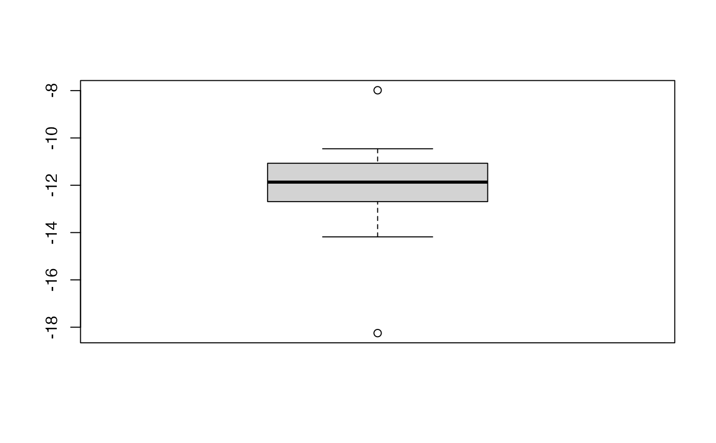 kfolds2Chisqind(bbb)
#> [[1]]
#> [[1]][[1]]
#> [1] NA NA NA NA NA NA NA NA NA NA
#>
#> [[1]][[2]]
#> [1] NA NA NA NA NA NA NA NA NA NA
#>
#> [[1]][[3]]
#> [1] NA NA NA NA NA NA NA NA NA NA
#>
#> [[1]][[4]]
#> [1] NA NA NA NA NA NA NA NA NA NA
#>
#> [[1]][[5]]
#> [1] NA NA NA NA NA NA NA NA NA NA
#>
#> [[1]][[6]]
#> [1] NA NA NA NA NA NA NA NA NA NA
#>
#> [[1]][[7]]
#> [1] NA NA NA NA NA NA NA NA NA NA
#>
#> [[1]][[8]]
#> [1] NA NA NA NA NA NA NA NA NA NA
#>
#> [[1]][[9]]
#> [1] NA NA NA NA NA NA NA NA NA NA
#>
#> [[1]][[10]]
#> [1] NA NA NA NA NA NA NA NA NA NA
#>
#>
kfolds2Chisq(bbb)
#> [[1]]
#> [1] NA NA NA NA NA NA NA NA NA NA
#>
summary(bbb)
#> ____************************************************____
#>
#> Family: Gamma
#> Link function: inverse
#>
#> ____Component____ 1 ____
#> ____Component____ 2 ____
#> ____Component____ 3 ____
#> ____Component____ 4 ____
#> ____Component____ 5 ____
#> ____Component____ 6 ____
#> ____Component____ 7 ____
#> ____Component____ 8 ____
#> ____Component____ 9 ____
#> ____Component____ 10 ____
#> ____Predicting X without NA neither in X or Y____
#> ****________________________________________________****
#>
#>
#> NK: 1
#> [[1]]
#> AIC BIC Q2Chisqcum_Y limQ2 Q2Chisq_Y PREChi2_Pearson_Y
#> Nb_Comp_0 56.60919 59.60220 NA NA NA NA
#> Nb_Comp_1 39.01090 43.50042 NA 0.0975 NA NA
#> Nb_Comp_2 37.30801 43.29404 NA 0.0975 NA NA
#> Nb_Comp_3 36.87524 44.35777 NA 0.0975 NA NA
#> Nb_Comp_4 36.55795 45.53700 NA 0.0975 NA NA
#> Nb_Comp_5 37.13611 47.61167 NA 0.0975 NA NA
#> Nb_Comp_6 38.27656 50.24862 NA 0.0975 NA NA
#> Nb_Comp_7 39.39377 52.86234 NA 0.0975 NA NA
#> Nb_Comp_8 40.96122 55.92630 NA 0.0975 NA NA
#> Nb_Comp_9 42.90816 59.36974 NA 0.0975 NA NA
#> Nb_Comp_10 44.90815 62.86625 NA 0.0975 NA NA
#> Chi2_Pearson_Y RSS_Y R2_Y
#> Nb_Comp_0 31.60805 20.800152 NA
#> Nb_Comp_1 17.31431 11.804594 0.4324756
#> Nb_Comp_2 17.01037 6.357437 0.6943562
#> Nb_Comp_3 15.83422 5.699662 0.7259798
#> Nb_Comp_4 13.52676 7.679741 0.6307844
#> Nb_Comp_5 13.60962 6.099077 0.7067773
#> Nb_Comp_6 13.91155 5.205052 0.7497590
#> Nb_Comp_7 14.94390 4.650377 0.7764258
#> Nb_Comp_8 15.25537 4.321314 0.7922461
#> Nb_Comp_9 15.15577 4.307757 0.7928978
#> Nb_Comp_10 15.15490 4.307391 0.7929154
#>
#> attr(,"class")
#> [1] "summary.cv.plsRglmmodel"
PLS_lm(ypine,Xpine,10,typeVC="standard")$InfCrit
#> ____************************************************____
#> ____TypeVC____ standard ____
#> ____Component____ 1 ____
#> ____Component____ 2 ____
#> ____Component____ 3 ____
#> ____Component____ 4 ____
#> ____Component____ 5 ____
#> ____Component____ 6 ____
#> ____Component____ 7 ____
#> ____Component____ 8 ____
#> ____Component____ 9 ____
#> ____Component____ 10 ____
#> ____Predicting X without NA neither in X nor in Y____
#> ****________________________________________________****
#>
#> AIC Q2cum_Y LimQ2_Y Q2_Y PRESS_Y RSS_Y
#> Nb_Comp_0 82.41888 NA NA NA NA 20.800152
#> Nb_Comp_1 63.61896 0.38248575 0.0975 0.38248575 12.844390 11.074659
#> Nb_Comp_2 58.47638 0.34836456 0.0975 -0.05525570 11.686597 8.919303
#> Nb_Comp_3 56.55421 0.23688359 0.0975 -0.17107874 10.445206 7.919786
#> Nb_Comp_4 54.35053 0.06999681 0.0975 -0.21869112 9.651773 6.972542
#> Nb_Comp_5 55.99834 -0.07691053 0.0975 -0.15796434 8.073955 6.898523
#> Nb_Comp_6 57.69592 -0.19968885 0.0975 -0.11400977 7.685022 6.835594
#> Nb_Comp_7 59.37953 -0.27722139 0.0975 -0.06462721 7.277359 6.770369
#> Nb_Comp_8 61.21213 -0.30602578 0.0975 -0.02255238 6.923057 6.736112
#> Nb_Comp_9 63.18426 -0.39920228 0.0975 -0.07134354 7.216690 6.730426
#> Nb_Comp_10 65.15982 -0.43743644 0.0975 -0.02732569 6.914340 6.725443
#> R2_Y R2_residY RSS_residY PRESS_residY Q2_residY LimQ2
#> Nb_Comp_0 NA NA 32.00000 NA NA NA
#> Nb_Comp_1 0.4675684 0.4675684 17.03781 19.76046 0.38248575 0.0975
#> Nb_Comp_2 0.5711905 0.5711905 13.72190 17.97925 -0.05525570 0.0975
#> Nb_Comp_3 0.6192438 0.6192438 12.18420 16.06943 -0.17107874 0.0975
#> Nb_Comp_4 0.6647841 0.6647841 10.72691 14.84877 -0.21869112 0.0975
#> Nb_Comp_5 0.6683426 0.6683426 10.61304 12.42138 -0.15796434 0.0975
#> Nb_Comp_6 0.6713681 0.6713681 10.51622 11.82303 -0.11400977 0.0975
#> Nb_Comp_7 0.6745039 0.6745039 10.41588 11.19586 -0.06462721 0.0975
#> Nb_Comp_8 0.6761508 0.6761508 10.36317 10.65078 -0.02255238 0.0975
#> Nb_Comp_9 0.6764242 0.6764242 10.35443 11.10252 -0.07134354 0.0975
#> Nb_Comp_10 0.6766638 0.6766638 10.34676 10.63737 -0.02732569 0.0975
#> Q2cum_residY AIC.std DoF.dof sigmahat.dof AIC.dof BIC.dof
#> Nb_Comp_0 NA 96.63448 1.000000 0.8062287 0.6697018 0.6991787
#> Nb_Comp_1 0.38248575 77.83455 3.176360 0.5994089 0.4047616 0.4565153
#> Nb_Comp_2 0.34836456 72.69198 7.133559 0.5761829 0.4138120 0.5212090
#> Nb_Comp_3 0.23688359 70.76981 8.778329 0.5603634 0.4070516 0.5320535
#> Nb_Comp_4 0.06999681 68.56612 8.427874 0.5221703 0.3505594 0.4547689
#> Nb_Comp_5 -0.07691053 70.21393 9.308247 0.5285695 0.3666578 0.4845912
#> Nb_Comp_6 -0.19968885 71.91152 9.291931 0.5259794 0.3629363 0.4795121
#> Nb_Comp_7 -0.27722139 73.59512 9.756305 0.5284535 0.3702885 0.4938445
#> Nb_Comp_8 -0.30602578 75.42772 10.363948 0.5338475 0.3831339 0.5170783
#> Nb_Comp_9 -0.39920228 77.39986 10.732145 0.5378276 0.3920956 0.5328746
#> Nb_Comp_10 -0.43743644 79.37542 11.000000 0.5407500 0.3987417 0.5446065
#> GMDL.dof DoF.naive sigmahat.naive AIC.naive BIC.naive GMDL.naive
#> Nb_Comp_0 -3.605128 1 0.8062287 0.6697018 0.6991787 -3.605128
#> Nb_Comp_1 -9.875081 2 0.5977015 0.3788984 0.4112998 -11.451340
#> Nb_Comp_2 -6.985517 3 0.5452615 0.3243383 0.3647862 -12.822703
#> Nb_Comp_3 -6.260610 4 0.5225859 0.3061986 0.3557368 -12.756838
#> Nb_Comp_4 -8.152986 5 0.4990184 0.2867496 0.3432131 -12.811575
#> Nb_Comp_5 -7.111583 6 0.5054709 0.3019556 0.3714754 -11.329638
#> Nb_Comp_6 -7.233043 7 0.5127450 0.3186757 0.4021333 -9.918688
#> Nb_Comp_7 -6.742195 8 0.5203986 0.3364668 0.4347156 -8.592770
#> Nb_Comp_8 -6.038372 9 0.5297842 0.3572181 0.4717708 -7.287834
#> Nb_Comp_9 -5.600238 10 0.5409503 0.3813021 0.5140048 -6.008747
#> Nb_Comp_10 -5.288422 11 0.5529032 0.4076026 0.5600977 -4.799453
data(pineNAX21)
bbb2 <- cv.plsRglm(x11~.,data=pineNAX21,nt=10,
modele="pls-glm-family",family=Gamma(),K=10,keepcoeffs=TRUE,keepfolds=FALSE,verbose=FALSE)
#> Warning: NaNs produced
#> Warning: NaNs produced
#> Warning: NaNs produced
bbb2 <- cv.plsRglm(x11~.,data=pineNAX21,nt=10,
modele="pls-glm-Gamma",K=10,keepcoeffs=TRUE,keepfolds=FALSE,verbose=FALSE)
#For Jackknife computations
kfolds2coeff(bbb2)
#> [,1] [,2] [,3] [,4] [,5] [,6]
#> [1,] -15.25147 0.006490479 0.04204947 -0.19442714 1.781305 -0.2952820
#> [2,] -15.16986 0.005474605 0.03527656 -0.27648100 1.257921 -0.2420263
#> [3,] -13.97006 0.010594537 -0.02927609 0.30604636 2.061606 -0.3365954
#> [4,] -12.03743 0.005373534 0.01951001 -0.08011735 1.311064 -0.2972826
#> [5,] -13.61994 0.005054427 0.01112295 -0.14897854 1.789084 -0.3465339
#> [6,] -14.86458 0.006538230 0.05144328 -0.19171348 1.762460 -0.3669618
#> [7,] -13.85270 0.006060799 0.06967588 -0.02328877 1.870853 -0.4052438
#> [8,] -14.36499 0.005602741 0.03767463 -0.16984964 1.754658 -0.3354075
#> [9,] -14.67958 0.006164958 0.05589650 -0.17300465 1.964310 -0.4224304
#> [10,] -15.30241 0.004702082 0.06265784 -0.28441615 2.354652 -0.5135518
#> [,7] [,8] [,9] [,10] [,11]
#> [1,] 2.5339085 -0.869322794 -0.50052940 1.5016832 1.1335442
#> [2,] 3.6679546 0.949554915 -0.27881465 1.4859881 0.7737842
#> [3,] -2.4661214 -0.929662624 -0.49572148 0.7713872 0.9698994
#> [4,] 1.1018507 -0.007227048 -0.02295972 0.5747632 0.6669312
#> [5,] 1.8359211 -0.272589375 -0.10305410 0.9830253 0.8989810
#> [6,] 2.8883524 -0.608454563 -0.18145293 0.2719423 0.7192753
#> [7,] -0.4468633 0.251324140 -0.03449214 1.2065942 0.0875273
#> [8,] 2.0699983 0.023096103 -0.21486194 1.1778879 0.3679135
#> [9,] 2.4902882 -0.580864643 -0.14887012 0.2397186 1.0540600
#> [10,] 3.5201888 -0.311832092 -0.18456971 1.1482720 0.6852035
boxplot(kfolds2coeff(bbb2)[,1])
kfolds2Chisqind(bbb)
#> [[1]]
#> [[1]][[1]]
#> [1] NA NA NA NA NA NA NA NA NA NA
#>
#> [[1]][[2]]
#> [1] NA NA NA NA NA NA NA NA NA NA
#>
#> [[1]][[3]]
#> [1] NA NA NA NA NA NA NA NA NA NA
#>
#> [[1]][[4]]
#> [1] NA NA NA NA NA NA NA NA NA NA
#>
#> [[1]][[5]]
#> [1] NA NA NA NA NA NA NA NA NA NA
#>
#> [[1]][[6]]
#> [1] NA NA NA NA NA NA NA NA NA NA
#>
#> [[1]][[7]]
#> [1] NA NA NA NA NA NA NA NA NA NA
#>
#> [[1]][[8]]
#> [1] NA NA NA NA NA NA NA NA NA NA
#>
#> [[1]][[9]]
#> [1] NA NA NA NA NA NA NA NA NA NA
#>
#> [[1]][[10]]
#> [1] NA NA NA NA NA NA NA NA NA NA
#>
#>
kfolds2Chisq(bbb)
#> [[1]]
#> [1] NA NA NA NA NA NA NA NA NA NA
#>
summary(bbb)
#> ____************************************************____
#>
#> Family: Gamma
#> Link function: inverse
#>
#> ____Component____ 1 ____
#> ____Component____ 2 ____
#> ____Component____ 3 ____
#> ____Component____ 4 ____
#> ____Component____ 5 ____
#> ____Component____ 6 ____
#> ____Component____ 7 ____
#> ____Component____ 8 ____
#> ____Component____ 9 ____
#> ____Component____ 10 ____
#> ____Predicting X without NA neither in X or Y____
#> ****________________________________________________****
#>
#>
#> NK: 1
#> [[1]]
#> AIC BIC Q2Chisqcum_Y limQ2 Q2Chisq_Y PREChi2_Pearson_Y
#> Nb_Comp_0 56.60919 59.60220 NA NA NA NA
#> Nb_Comp_1 39.01090 43.50042 NA 0.0975 NA NA
#> Nb_Comp_2 37.30801 43.29404 NA 0.0975 NA NA
#> Nb_Comp_3 36.87524 44.35777 NA 0.0975 NA NA
#> Nb_Comp_4 36.55795 45.53700 NA 0.0975 NA NA
#> Nb_Comp_5 37.13611 47.61167 NA 0.0975 NA NA
#> Nb_Comp_6 38.27656 50.24862 NA 0.0975 NA NA
#> Nb_Comp_7 39.39377 52.86234 NA 0.0975 NA NA
#> Nb_Comp_8 40.96122 55.92630 NA 0.0975 NA NA
#> Nb_Comp_9 42.90816 59.36974 NA 0.0975 NA NA
#> Nb_Comp_10 44.90815 62.86625 NA 0.0975 NA NA
#> Chi2_Pearson_Y RSS_Y R2_Y
#> Nb_Comp_0 31.60805 20.800152 NA
#> Nb_Comp_1 17.31431 11.804594 0.4324756
#> Nb_Comp_2 17.01037 6.357437 0.6943562
#> Nb_Comp_3 15.83422 5.699662 0.7259798
#> Nb_Comp_4 13.52676 7.679741 0.6307844
#> Nb_Comp_5 13.60962 6.099077 0.7067773
#> Nb_Comp_6 13.91155 5.205052 0.7497590
#> Nb_Comp_7 14.94390 4.650377 0.7764258
#> Nb_Comp_8 15.25537 4.321314 0.7922461
#> Nb_Comp_9 15.15577 4.307757 0.7928978
#> Nb_Comp_10 15.15490 4.307391 0.7929154
#>
#> attr(,"class")
#> [1] "summary.cv.plsRglmmodel"
PLS_lm(ypine,Xpine,10,typeVC="standard")$InfCrit
#> ____************************************************____
#> ____TypeVC____ standard ____
#> ____Component____ 1 ____
#> ____Component____ 2 ____
#> ____Component____ 3 ____
#> ____Component____ 4 ____
#> ____Component____ 5 ____
#> ____Component____ 6 ____
#> ____Component____ 7 ____
#> ____Component____ 8 ____
#> ____Component____ 9 ____
#> ____Component____ 10 ____
#> ____Predicting X without NA neither in X nor in Y____
#> ****________________________________________________****
#>
#> AIC Q2cum_Y LimQ2_Y Q2_Y PRESS_Y RSS_Y
#> Nb_Comp_0 82.41888 NA NA NA NA 20.800152
#> Nb_Comp_1 63.61896 0.38248575 0.0975 0.38248575 12.844390 11.074659
#> Nb_Comp_2 58.47638 0.34836456 0.0975 -0.05525570 11.686597 8.919303
#> Nb_Comp_3 56.55421 0.23688359 0.0975 -0.17107874 10.445206 7.919786
#> Nb_Comp_4 54.35053 0.06999681 0.0975 -0.21869112 9.651773 6.972542
#> Nb_Comp_5 55.99834 -0.07691053 0.0975 -0.15796434 8.073955 6.898523
#> Nb_Comp_6 57.69592 -0.19968885 0.0975 -0.11400977 7.685022 6.835594
#> Nb_Comp_7 59.37953 -0.27722139 0.0975 -0.06462721 7.277359 6.770369
#> Nb_Comp_8 61.21213 -0.30602578 0.0975 -0.02255238 6.923057 6.736112
#> Nb_Comp_9 63.18426 -0.39920228 0.0975 -0.07134354 7.216690 6.730426
#> Nb_Comp_10 65.15982 -0.43743644 0.0975 -0.02732569 6.914340 6.725443
#> R2_Y R2_residY RSS_residY PRESS_residY Q2_residY LimQ2
#> Nb_Comp_0 NA NA 32.00000 NA NA NA
#> Nb_Comp_1 0.4675684 0.4675684 17.03781 19.76046 0.38248575 0.0975
#> Nb_Comp_2 0.5711905 0.5711905 13.72190 17.97925 -0.05525570 0.0975
#> Nb_Comp_3 0.6192438 0.6192438 12.18420 16.06943 -0.17107874 0.0975
#> Nb_Comp_4 0.6647841 0.6647841 10.72691 14.84877 -0.21869112 0.0975
#> Nb_Comp_5 0.6683426 0.6683426 10.61304 12.42138 -0.15796434 0.0975
#> Nb_Comp_6 0.6713681 0.6713681 10.51622 11.82303 -0.11400977 0.0975
#> Nb_Comp_7 0.6745039 0.6745039 10.41588 11.19586 -0.06462721 0.0975
#> Nb_Comp_8 0.6761508 0.6761508 10.36317 10.65078 -0.02255238 0.0975
#> Nb_Comp_9 0.6764242 0.6764242 10.35443 11.10252 -0.07134354 0.0975
#> Nb_Comp_10 0.6766638 0.6766638 10.34676 10.63737 -0.02732569 0.0975
#> Q2cum_residY AIC.std DoF.dof sigmahat.dof AIC.dof BIC.dof
#> Nb_Comp_0 NA 96.63448 1.000000 0.8062287 0.6697018 0.6991787
#> Nb_Comp_1 0.38248575 77.83455 3.176360 0.5994089 0.4047616 0.4565153
#> Nb_Comp_2 0.34836456 72.69198 7.133559 0.5761829 0.4138120 0.5212090
#> Nb_Comp_3 0.23688359 70.76981 8.778329 0.5603634 0.4070516 0.5320535
#> Nb_Comp_4 0.06999681 68.56612 8.427874 0.5221703 0.3505594 0.4547689
#> Nb_Comp_5 -0.07691053 70.21393 9.308247 0.5285695 0.3666578 0.4845912
#> Nb_Comp_6 -0.19968885 71.91152 9.291931 0.5259794 0.3629363 0.4795121
#> Nb_Comp_7 -0.27722139 73.59512 9.756305 0.5284535 0.3702885 0.4938445
#> Nb_Comp_8 -0.30602578 75.42772 10.363948 0.5338475 0.3831339 0.5170783
#> Nb_Comp_9 -0.39920228 77.39986 10.732145 0.5378276 0.3920956 0.5328746
#> Nb_Comp_10 -0.43743644 79.37542 11.000000 0.5407500 0.3987417 0.5446065
#> GMDL.dof DoF.naive sigmahat.naive AIC.naive BIC.naive GMDL.naive
#> Nb_Comp_0 -3.605128 1 0.8062287 0.6697018 0.6991787 -3.605128
#> Nb_Comp_1 -9.875081 2 0.5977015 0.3788984 0.4112998 -11.451340
#> Nb_Comp_2 -6.985517 3 0.5452615 0.3243383 0.3647862 -12.822703
#> Nb_Comp_3 -6.260610 4 0.5225859 0.3061986 0.3557368 -12.756838
#> Nb_Comp_4 -8.152986 5 0.4990184 0.2867496 0.3432131 -12.811575
#> Nb_Comp_5 -7.111583 6 0.5054709 0.3019556 0.3714754 -11.329638
#> Nb_Comp_6 -7.233043 7 0.5127450 0.3186757 0.4021333 -9.918688
#> Nb_Comp_7 -6.742195 8 0.5203986 0.3364668 0.4347156 -8.592770
#> Nb_Comp_8 -6.038372 9 0.5297842 0.3572181 0.4717708 -7.287834
#> Nb_Comp_9 -5.600238 10 0.5409503 0.3813021 0.5140048 -6.008747
#> Nb_Comp_10 -5.288422 11 0.5529032 0.4076026 0.5600977 -4.799453
data(pineNAX21)
bbb2 <- cv.plsRglm(x11~.,data=pineNAX21,nt=10,
modele="pls-glm-family",family=Gamma(),K=10,keepcoeffs=TRUE,keepfolds=FALSE,verbose=FALSE)
#> Warning: NaNs produced
#> Warning: NaNs produced
#> Warning: NaNs produced
bbb2 <- cv.plsRglm(x11~.,data=pineNAX21,nt=10,
modele="pls-glm-Gamma",K=10,keepcoeffs=TRUE,keepfolds=FALSE,verbose=FALSE)
#For Jackknife computations
kfolds2coeff(bbb2)
#> [,1] [,2] [,3] [,4] [,5] [,6]
#> [1,] -15.25147 0.006490479 0.04204947 -0.19442714 1.781305 -0.2952820
#> [2,] -15.16986 0.005474605 0.03527656 -0.27648100 1.257921 -0.2420263
#> [3,] -13.97006 0.010594537 -0.02927609 0.30604636 2.061606 -0.3365954
#> [4,] -12.03743 0.005373534 0.01951001 -0.08011735 1.311064 -0.2972826
#> [5,] -13.61994 0.005054427 0.01112295 -0.14897854 1.789084 -0.3465339
#> [6,] -14.86458 0.006538230 0.05144328 -0.19171348 1.762460 -0.3669618
#> [7,] -13.85270 0.006060799 0.06967588 -0.02328877 1.870853 -0.4052438
#> [8,] -14.36499 0.005602741 0.03767463 -0.16984964 1.754658 -0.3354075
#> [9,] -14.67958 0.006164958 0.05589650 -0.17300465 1.964310 -0.4224304
#> [10,] -15.30241 0.004702082 0.06265784 -0.28441615 2.354652 -0.5135518
#> [,7] [,8] [,9] [,10] [,11]
#> [1,] 2.5339085 -0.869322794 -0.50052940 1.5016832 1.1335442
#> [2,] 3.6679546 0.949554915 -0.27881465 1.4859881 0.7737842
#> [3,] -2.4661214 -0.929662624 -0.49572148 0.7713872 0.9698994
#> [4,] 1.1018507 -0.007227048 -0.02295972 0.5747632 0.6669312
#> [5,] 1.8359211 -0.272589375 -0.10305410 0.9830253 0.8989810
#> [6,] 2.8883524 -0.608454563 -0.18145293 0.2719423 0.7192753
#> [7,] -0.4468633 0.251324140 -0.03449214 1.2065942 0.0875273
#> [8,] 2.0699983 0.023096103 -0.21486194 1.1778879 0.3679135
#> [9,] 2.4902882 -0.580864643 -0.14887012 0.2397186 1.0540600
#> [10,] 3.5201888 -0.311832092 -0.18456971 1.1482720 0.6852035
boxplot(kfolds2coeff(bbb2)[,1])
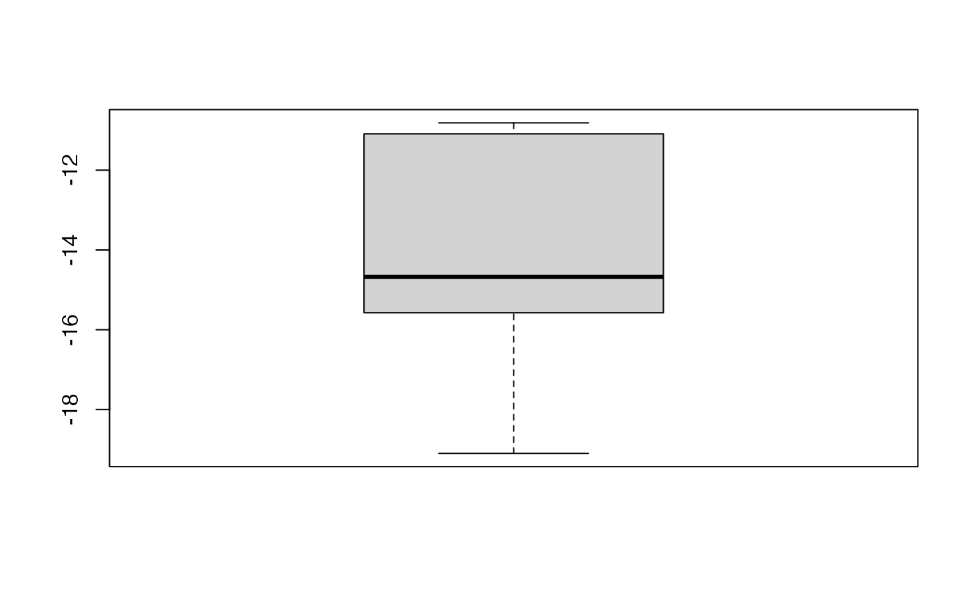 kfolds2Chisqind(bbb2)
#> [[1]]
#> [[1]][[1]]
#> [1] NA NA NA NA NA NA NA NA NA
#>
#> [[1]][[2]]
#> [1] NA NA NA NA NA NA NA NA NA
#>
#> [[1]][[3]]
#> [1] NA NA NA NA NA NA NA NA NA
#>
#> [[1]][[4]]
#> [1] NA NA NA NA NA NA NA NA NA
#>
#> [[1]][[5]]
#> [1] NA NA NA NA NA NA NA NA NA
#>
#> [[1]][[6]]
#> [1] NA NA NA NA NA NA NA NA NA
#>
#> [[1]][[7]]
#> [1] NA NA NA NA NA NA NA NA NA
#>
#> [[1]][[8]]
#> [1] NA NA NA NA NA NA NA NA NA
#>
#> [[1]][[9]]
#> [1] NA NA NA NA NA NA NA NA NA
#>
#> [[1]][[10]]
#> [1] NA NA NA NA NA NA NA NA NA
#>
#>
kfolds2Chisq(bbb2)
#> [[1]]
#> [1] NA NA NA NA NA NA NA NA NA
#>
summary(bbb2)
#> ____************************************************____
#> Only naive DoF can be used with missing data
#>
#> Family: Gamma
#> Link function: inverse
#>
#> ____There are some NAs in X but not in Y____
#> ____Component____ 1 ____
#> ____Component____ 2 ____
#> ____Component____ 3 ____
#> ____Component____ 4 ____
#> ____Component____ 5 ____
#> ____Component____ 6 ____
#> ____Component____ 7 ____
#> ____Component____ 8 ____
#> ____Component____ 9 ____
#> ____Predicting X with NA in X and not in Y____
#> ****________________________________________________****
#>
#>
#> NK: 1
#> [[1]]
#> AIC BIC Q2Chisqcum_Y limQ2 Q2Chisq_Y PREChi2_Pearson_Y
#> Nb_Comp_0 56.60919 59.60220 NA NA NA NA
#> Nb_Comp_1 39.08940 43.57892 NA 0.0975 NA NA
#> Nb_Comp_2 37.36154 43.34757 NA 0.0975 NA NA
#> Nb_Comp_3 36.81173 44.29427 NA 0.0975 NA NA
#> Nb_Comp_4 36.53654 45.51559 NA 0.0975 NA NA
#> Nb_Comp_5 37.24312 47.71867 NA 0.0975 NA NA
#> Nb_Comp_6 38.18649 50.15855 NA 0.0975 NA NA
#> Nb_Comp_7 39.35575 52.82432 NA 0.0975 NA NA
#> Nb_Comp_8 40.86209 55.82716 NA 0.0975 NA NA
#> Nb_Comp_9 42.80511 59.26669 NA 0.0975 NA NA
#> Chi2_Pearson_Y RSS_Y R2_Y
#> Nb_Comp_0 31.60805 20.800152 NA
#> Nb_Comp_1 17.30890 12.031518 0.4215659
#> Nb_Comp_2 17.10360 6.183372 0.7027247
#> Nb_Comp_3 15.78579 5.756462 0.7232490
#> Nb_Comp_4 13.49013 7.630460 0.6331536
#> Nb_Comp_5 13.56918 6.303455 0.6969515
#> Nb_Comp_6 14.02295 5.274716 0.7464097
#> Nb_Comp_7 15.05896 4.867806 0.7659726
#> Nb_Comp_8 15.28052 4.317488 0.7924300
#> Nb_Comp_9 15.19429 4.298593 0.7933384
#>
#> attr(,"class")
#> [1] "summary.cv.plsRglmmodel"
XpineNAX21 <- Xpine
XpineNAX21[1,2] <- NA
PLS_lm(ypine,XpineNAX21,10,typeVC="standard")$InfCrit
#> ____************************************************____
#> Only naive DoF can be used with missing data
#> ____There are some NAs in X but not in Y____
#> ____TypeVC____ standard ____
#> ____Component____ 1 ____
#> ____Component____ 2 ____
#> ____Component____ 3 ____
#> ____Component____ 4 ____
#> ____Component____ 5 ____
#> ____Component____ 6 ____
#> ____Component____ 7 ____
#> ____Component____ 8 ____
#> ____Component____ 9 ____
#> Warning : reciprocal condition number of t(cbind(res$pp,temppp)[XXNA[1,],,drop=FALSE])%*%cbind(res$pp,temppp)[XXNA[1,],,drop=FALSE] < 10^{-12}
#> Warning only 9 components could thus be extracted
#> ____Predicting X with NA in X and not in Y____
#> ****________________________________________________****
#>
#> AIC Q2cum_Y LimQ2_Y Q2_Y PRESS_Y RSS_Y
#> Nb_Comp_0 82.41888 NA NA NA NA 20.800152
#> Nb_Comp_1 63.69250 0.35639805 0.0975 0.35639805 13.387018 11.099368
#> Nb_Comp_2 58.35228 0.28395028 0.0975 -0.11256611 12.348781 8.885823
#> Nb_Comp_3 56.36553 0.07664889 0.0975 -0.28950699 11.458331 7.874634
#> Nb_Comp_4 54.02416 -0.70355579 0.0975 -0.84497074 14.528469 6.903925
#> Nb_Comp_5 55.80450 -0.94905654 0.0975 -0.14411078 7.898855 6.858120
#> Nb_Comp_6 57.45753 -1.27568315 0.0975 -0.16758190 8.007417 6.786392
#> Nb_Comp_7 58.73951 -1.63309014 0.0975 -0.15705481 7.852227 6.640327
#> Nb_Comp_8 60.61227 -1.67907859 0.0975 -0.01746558 6.756304 6.614773
#> Nb_Comp_9 62.25948 -2.15165796 0.0975 -0.17639623 7.781594 6.544432
#> R2_Y R2_residY RSS_residY PRESS_residY Q2_residY LimQ2
#> Nb_Comp_0 NA NA 32.00000 NA NA NA
#> Nb_Comp_1 0.4663804 0.4663804 17.07583 20.59526 0.35639805 0.0975
#> Nb_Comp_2 0.5728001 0.5728001 13.67040 18.99799 -0.11256611 0.0975
#> Nb_Comp_3 0.6214146 0.6214146 12.11473 17.62807 -0.28950699 0.0975
#> Nb_Comp_4 0.6680830 0.6680830 10.62135 22.35133 -0.84497074 0.0975
#> Nb_Comp_5 0.6702851 0.6702851 10.55088 12.15200 -0.14411078 0.0975
#> Nb_Comp_6 0.6737336 0.6737336 10.44053 12.31901 -0.16758190 0.0975
#> Nb_Comp_7 0.6807558 0.6807558 10.21581 12.08026 -0.15705481 0.0975
#> Nb_Comp_8 0.6819844 0.6819844 10.17650 10.39424 -0.01746558 0.0975
#> Nb_Comp_9 0.6853661 0.6853661 10.06828 11.97160 -0.17639623 0.0975
#> Q2cum_residY AIC.std DoF.dof sigmahat.dof AIC.dof BIC.dof GMDL.dof
#> Nb_Comp_0 NA 96.63448 NA NA NA NA NA
#> Nb_Comp_1 0.35639805 77.90810 NA NA NA NA NA
#> Nb_Comp_2 0.28395028 72.56787 NA NA NA NA NA
#> Nb_Comp_3 0.07664889 70.58113 NA NA NA NA NA
#> Nb_Comp_4 -0.70355579 68.23976 NA NA NA NA NA
#> Nb_Comp_5 -0.94905654 70.02009 NA NA NA NA NA
#> Nb_Comp_6 -1.27568315 71.67313 NA NA NA NA NA
#> Nb_Comp_7 -1.63309014 72.95511 NA NA NA NA NA
#> Nb_Comp_8 -1.67907859 74.82787 NA NA NA NA NA
#> Nb_Comp_9 -2.15165796 76.47507 NA NA NA NA NA
#> DoF.naive sigmahat.naive AIC.naive BIC.naive GMDL.naive
#> Nb_Comp_0 1 0.8062287 0.6697018 0.6991787 -3.605128
#> Nb_Comp_1 2 0.5983679 0.3797438 0.4122175 -11.413749
#> Nb_Comp_2 3 0.5442372 0.3231208 0.3634169 -12.847656
#> Nb_Comp_3 4 0.5210941 0.3044529 0.3537087 -12.776843
#> Nb_Comp_4 5 0.4965569 0.2839276 0.3398355 -12.891035
#> Nb_Comp_5 6 0.5039885 0.3001871 0.3692997 -11.349498
#> Nb_Comp_6 7 0.5108963 0.3163819 0.3992388 -9.922119
#> Nb_Comp_7 8 0.5153766 0.3300041 0.4263658 -8.696873
#> Nb_Comp_8 9 0.5249910 0.3507834 0.4632727 -7.337679
#> Nb_Comp_9 10 0.5334234 0.3707649 0.4998004 -6.033403
rm(list=c("Xpine","XpineNAX21","ypine","bbb","bbb2"))
data(Cornell)
XCornell<-Cornell[,1:7]
yCornell<-Cornell[,8]
bbb <- cv.plsRglm(Y~.,data=Cornell,nt=10,NK=1,modele="pls",verbose=FALSE)
summary(bbb)
#> ____************************************************____
#>
#> Model: pls
#>
#> ____Component____ 1 ____
#> ____Component____ 2 ____
#> ____Component____ 3 ____
#> ____Component____ 4 ____
#> ____Component____ 5 ____
#> ____Component____ 6 ____
#> ____Predicting X without NA neither in X or Y____
#> ****________________________________________________****
#>
#>
#> NK: 1
#> [[1]]
#> AIC Q2cum_Y LimQ2_Y Q2_Y PRESS_Y RSS_Y R2_Y
#> Nb_Comp_0 82.01205 NA NA NA NA 467.796667 NA
#> Nb_Comp_1 53.15173 0.8375127 0.0975 0.8375127 76.01101 35.742486 0.9235940
#> Nb_Comp_2 41.08283 0.7843768 0.0975 -0.3270158 47.43084 11.066606 0.9763431
#> Nb_Comp_3 32.06411 0.3361792 0.0975 -2.0786151 34.06982 4.418081 0.9905556
#> Nb_Comp_4 33.76477 -5.7521467 0.0975 -9.1716408 44.93914 4.309235 0.9907882
#> Nb_Comp_5 33.34373 -64.2459132 0.0975 -8.6629881 41.64009 3.521924 0.9924713
#> Nb_Comp_6 35.25533 NA 0.0975 NA NA 3.496074 0.9925265
#> AIC.std DoF.dof sigmahat.dof AIC.dof BIC.dof GMDL.dof
#> Nb_Comp_0 37.010388 1.000000 6.5212706 46.0708838 47.7893514 27.59461
#> Nb_Comp_1 8.150064 2.740749 1.8665281 4.5699686 4.9558156 21.34020
#> Nb_Comp_2 -3.918831 5.085967 1.1825195 2.1075461 2.3949331 27.40202
#> Nb_Comp_3 -12.937550 5.121086 0.7488308 0.8467795 0.9628191 24.40842
#> Nb_Comp_4 -11.236891 5.103312 0.7387162 0.8232505 0.9357846 24.23105
#> Nb_Comp_5 -11.657929 6.006316 0.7096382 0.7976101 0.9198348 28.21184
#> Nb_Comp_6 -9.746328 7.000002 0.7633343 0.9711321 1.1359501 33.18347
#> DoF.naive sigmahat.naive AIC.naive BIC.naive GMDL.naive
#> Nb_Comp_0 1 6.5212706 46.0708838 47.7893514 27.59461
#> Nb_Comp_1 2 1.8905683 4.1699567 4.4588195 18.37545
#> Nb_Comp_2 3 1.1088836 1.5370286 1.6860917 17.71117
#> Nb_Comp_3 4 0.7431421 0.7363469 0.8256118 19.01033
#> Nb_Comp_4 5 0.7846050 0.8721072 0.9964867 24.16510
#> Nb_Comp_5 6 0.7661509 0.8804809 1.0227979 28.64206
#> Nb_Comp_6 7 0.8361907 1.1070902 1.3048716 33.63927
#>
#> attr(,"class")
#> [1] "summary.cv.plsRmodel"
cv.plsRglm(object=yCornell,dataX=XCornell,nt=3,modele="pls-glm-inverse.gaussian",K=12,verbose=FALSE)
#> Number of repeated crossvalidations:
#> [1] 1
#> Number of folds for each crossvalidation:
#> [1] 12
cv.plsRglm(object=yCornell,dataX=XCornell,nt=3,modele="pls-glm-family",
family=inverse.gaussian,K=12,verbose=FALSE)
#> Number of repeated crossvalidations:
#> [1] 1
#> Number of folds for each crossvalidation:
#> [1] 12
cv.plsRglm(object=yCornell,dataX=XCornell,nt=3,modele="pls-glm-inverse.gaussian",K=6,
NK=2,verbose=FALSE)$results_kfolds
#> [[1]]
#> [[1]][[1]]
#> [,1] [,2] [,3]
#> 2 NA NA NA
#> 1 NA NA NA
#>
#> [[1]][[2]]
#> [,1] [,2] [,3]
#> 11 NA NA NA
#> 12 NA NA NA
#>
#> [[1]][[3]]
#> [,1] [,2] [,3]
#> 10 NA NA NA
#> 8 NA NA NA
#>
#> [[1]][[4]]
#> [,1] [,2] [,3]
#> 7 NA NA NA
#> 9 NA NA NA
#>
#> [[1]][[5]]
#> [,1] [,2] [,3]
#> 3 NA NA NA
#> 6 NA NA NA
#>
#> [[1]][[6]]
#> [,1] [,2] [,3]
#> 4 NA NA NA
#> 5 NA NA NA
#>
#>
#> [[2]]
#> [[2]][[1]]
#> [,1] [,2] [,3]
#> 5 NA NA NA
#> 3 NA NA NA
#>
#> [[2]][[2]]
#> [,1] [,2] [,3]
#> 6 NA NA NA
#> 11 NA NA NA
#>
#> [[2]][[3]]
#> [,1] [,2] [,3]
#> 2 NA NA NA
#> 1 NA NA NA
#>
#> [[2]][[4]]
#> [,1] [,2] [,3]
#> 8 NA NA NA
#> 12 NA NA NA
#>
#> [[2]][[5]]
#> [,1] [,2] [,3]
#> 7 NA NA NA
#> 10 NA NA NA
#>
#> [[2]][[6]]
#> [,1] [,2] [,3]
#> 4 NA NA NA
#> 9 NA NA NA
#>
#>
cv.plsRglm(object=yCornell,dataX=XCornell,nt=3,modele="pls-glm-family",family=inverse.gaussian(),
K=6,NK=2,verbose=FALSE)$results_kfolds
#> [[1]]
#> [[1]][[1]]
#> [,1] [,2] [,3]
#> 2 NA NA NA
#> 6 NA NA NA
#>
#> [[1]][[2]]
#> [,1] [,2] [,3]
#> 11 NA NA NA
#> 12 NA NA NA
#>
#> [[1]][[3]]
#> [,1] [,2] [,3]
#> 5 NA NA NA
#> 10 NA NA NA
#>
#> [[1]][[4]]
#> [,1] [,2] [,3]
#> 3 NA NA NA
#> 8 NA NA NA
#>
#> [[1]][[5]]
#> [,1] [,2] [,3]
#> 1 NA NA NA
#> 9 NA NA NA
#>
#> [[1]][[6]]
#> [,1] [,2] [,3]
#> 4 NA NA NA
#> 7 NA NA NA
#>
#>
#> [[2]]
#> [[2]][[1]]
#> [,1] [,2] [,3]
#> 10 NA NA NA
#> 11 NA NA NA
#>
#> [[2]][[2]]
#> [,1] [,2] [,3]
#> 5 NA NA NA
#> 8 NA NA NA
#>
#> [[2]][[3]]
#> [,1] [,2] [,3]
#> 12 NA NA NA
#> 1 NA NA NA
#>
#> [[2]][[4]]
#> [,1] [,2] [,3]
#> 4 NA NA NA
#> 9 NA NA NA
#>
#> [[2]][[5]]
#> [,1] [,2] [,3]
#> 7 NA NA NA
#> 6 NA NA NA
#>
#> [[2]][[6]]
#> [,1] [,2] [,3]
#> 3 NA NA NA
#> 2 NA NA NA
#>
#>
cv.plsRglm(object=yCornell,dataX=XCornell,nt=3,modele="pls-glm-inverse.gaussian",K=6,
NK=2,verbose=FALSE)$results_kfolds
#> [[1]]
#> [[1]][[1]]
#> [,1] [,2] [,3]
#> 9 NA NA NA
#> 10 NA NA NA
#>
#> [[1]][[2]]
#> [,1] [,2] [,3]
#> 4 NA NA NA
#> 12 NA NA NA
#>
#> [[1]][[3]]
#> [,1] [,2] [,3]
#> 2 NA NA NA
#> 1 NA NA NA
#>
#> [[1]][[4]]
#> [,1] [,2] [,3]
#> 6 NA NA NA
#> 7 NA NA NA
#>
#> [[1]][[5]]
#> [,1] [,2] [,3]
#> 5 NA NA NA
#> 8 NA NA NA
#>
#> [[1]][[6]]
#> [,1] [,2] [,3]
#> 3 NA NA NA
#> 11 NA NA NA
#>
#>
#> [[2]]
#> [[2]][[1]]
#> [,1] [,2] [,3]
#> 5 NA NA NA
#> 2 NA NA NA
#>
#> [[2]][[2]]
#> [,1] [,2] [,3]
#> 4 NA NA NA
#> 12 NA NA NA
#>
#> [[2]][[3]]
#> [,1] [,2] [,3]
#> 3 NA NA NA
#> 7 NA NA NA
#>
#> [[2]][[4]]
#> [,1] [,2] [,3]
#> 8 NA NA NA
#> 11 NA NA NA
#>
#> [[2]][[5]]
#> [,1] [,2] [,3]
#> 9 NA NA NA
#> 10 NA NA NA
#>
#> [[2]][[6]]
#> [,1] [,2] [,3]
#> 1 NA NA NA
#> 6 NA NA NA
#>
#>
cv.plsRglm(object=yCornell,dataX=XCornell,nt=3,modele="pls-glm-family",
family=inverse.gaussian(link = "1/mu^2"),K=6,NK=2,verbose=FALSE)$results_kfolds
#> [[1]]
#> [[1]][[1]]
#> [,1] [,2] [,3]
#> 3 NA NA NA
#> 7 NA NA NA
#>
#> [[1]][[2]]
#> [,1] [,2] [,3]
#> 8 NA NA NA
#> 1 NA NA NA
#>
#> [[1]][[3]]
#> [,1] [,2] [,3]
#> 5 NA NA NA
#> 10 NA NA NA
#>
#> [[1]][[4]]
#> [,1] [,2] [,3]
#> 12 NA NA NA
#> 4 NA NA NA
#>
#> [[1]][[5]]
#> [,1] [,2] [,3]
#> 9 NA NA NA
#> 6 NA NA NA
#>
#> [[1]][[6]]
#> [,1] [,2] [,3]
#> 2 NA NA NA
#> 11 NA NA NA
#>
#>
#> [[2]]
#> [[2]][[1]]
#> [,1] [,2] [,3]
#> 2 NA NA NA
#> 8 NA NA NA
#>
#> [[2]][[2]]
#> [,1] [,2] [,3]
#> 6 NA NA NA
#> 10 NA NA NA
#>
#> [[2]][[3]]
#> [,1] [,2] [,3]
#> 12 NA NA NA
#> 9 NA NA NA
#>
#> [[2]][[4]]
#> [,1] [,2] [,3]
#> 3 NA NA NA
#> 4 NA NA NA
#>
#> [[2]][[5]]
#> [,1] [,2] [,3]
#> 5 NA NA NA
#> 7 NA NA NA
#>
#> [[2]][[6]]
#> [,1] [,2] [,3]
#> 11 NA NA NA
#> 1 NA NA NA
#>
#>
bbb2 <- cv.plsRglm(Y~.,data=Cornell,nt=10,
modele="pls-glm-inverse.gaussian",keepcoeffs=TRUE,verbose=FALSE)
#For Jackknife computations
kfolds2coeff(bbb2)
#> [,1] [,2] [,3] [,4] [,5]
#> [1,] 0.0002136666 -3.152061e-05 -8.004098e-05 -5.358504e-05 -4.875042e-05
#> [2,] 0.0024298065 -3.505496e-03 -2.306928e-03 3.172305e-04 -2.115984e-03
#> [3,] 0.0001395896 2.587855e-04 -6.570595e-06 -3.435778e-04 1.261472e-05
#> [4,] -0.0019335956 2.585441e-03 2.063289e-03 1.273572e-03 2.075435e-03
#> [5,] -0.0001726175 7.866832e-04 3.087020e-04 -4.618726e-04 3.028237e-04
#> [,6] [,7] [,8]
#> [1,] -6.981066e-05 -1.163207e-04 -1.863569e-04
#> [2,] -2.324571e-03 -2.277295e-03 -3.688473e-03
#> [3,] -2.704572e-05 -3.926685e-05 -4.286597e-05
#> [4,] 2.065248e-03 2.026394e-03 2.118389e-03
#> [5,] 2.972386e-04 2.591324e-04 4.486940e-04
boxplot(kfolds2coeff(bbb2)[,1])
kfolds2Chisqind(bbb2)
#> [[1]]
#> [[1]][[1]]
#> [1] NA NA NA NA NA NA NA NA NA
#>
#> [[1]][[2]]
#> [1] NA NA NA NA NA NA NA NA NA
#>
#> [[1]][[3]]
#> [1] NA NA NA NA NA NA NA NA NA
#>
#> [[1]][[4]]
#> [1] NA NA NA NA NA NA NA NA NA
#>
#> [[1]][[5]]
#> [1] NA NA NA NA NA NA NA NA NA
#>
#> [[1]][[6]]
#> [1] NA NA NA NA NA NA NA NA NA
#>
#> [[1]][[7]]
#> [1] NA NA NA NA NA NA NA NA NA
#>
#> [[1]][[8]]
#> [1] NA NA NA NA NA NA NA NA NA
#>
#> [[1]][[9]]
#> [1] NA NA NA NA NA NA NA NA NA
#>
#> [[1]][[10]]
#> [1] NA NA NA NA NA NA NA NA NA
#>
#>
kfolds2Chisq(bbb2)
#> [[1]]
#> [1] NA NA NA NA NA NA NA NA NA
#>
summary(bbb2)
#> ____************************************************____
#> Only naive DoF can be used with missing data
#>
#> Family: Gamma
#> Link function: inverse
#>
#> ____There are some NAs in X but not in Y____
#> ____Component____ 1 ____
#> ____Component____ 2 ____
#> ____Component____ 3 ____
#> ____Component____ 4 ____
#> ____Component____ 5 ____
#> ____Component____ 6 ____
#> ____Component____ 7 ____
#> ____Component____ 8 ____
#> ____Component____ 9 ____
#> ____Predicting X with NA in X and not in Y____
#> ****________________________________________________****
#>
#>
#> NK: 1
#> [[1]]
#> AIC BIC Q2Chisqcum_Y limQ2 Q2Chisq_Y PREChi2_Pearson_Y
#> Nb_Comp_0 56.60919 59.60220 NA NA NA NA
#> Nb_Comp_1 39.08940 43.57892 NA 0.0975 NA NA
#> Nb_Comp_2 37.36154 43.34757 NA 0.0975 NA NA
#> Nb_Comp_3 36.81173 44.29427 NA 0.0975 NA NA
#> Nb_Comp_4 36.53654 45.51559 NA 0.0975 NA NA
#> Nb_Comp_5 37.24312 47.71867 NA 0.0975 NA NA
#> Nb_Comp_6 38.18649 50.15855 NA 0.0975 NA NA
#> Nb_Comp_7 39.35575 52.82432 NA 0.0975 NA NA
#> Nb_Comp_8 40.86209 55.82716 NA 0.0975 NA NA
#> Nb_Comp_9 42.80511 59.26669 NA 0.0975 NA NA
#> Chi2_Pearson_Y RSS_Y R2_Y
#> Nb_Comp_0 31.60805 20.800152 NA
#> Nb_Comp_1 17.30890 12.031518 0.4215659
#> Nb_Comp_2 17.10360 6.183372 0.7027247
#> Nb_Comp_3 15.78579 5.756462 0.7232490
#> Nb_Comp_4 13.49013 7.630460 0.6331536
#> Nb_Comp_5 13.56918 6.303455 0.6969515
#> Nb_Comp_6 14.02295 5.274716 0.7464097
#> Nb_Comp_7 15.05896 4.867806 0.7659726
#> Nb_Comp_8 15.28052 4.317488 0.7924300
#> Nb_Comp_9 15.19429 4.298593 0.7933384
#>
#> attr(,"class")
#> [1] "summary.cv.plsRglmmodel"
XpineNAX21 <- Xpine
XpineNAX21[1,2] <- NA
PLS_lm(ypine,XpineNAX21,10,typeVC="standard")$InfCrit
#> ____************************************************____
#> Only naive DoF can be used with missing data
#> ____There are some NAs in X but not in Y____
#> ____TypeVC____ standard ____
#> ____Component____ 1 ____
#> ____Component____ 2 ____
#> ____Component____ 3 ____
#> ____Component____ 4 ____
#> ____Component____ 5 ____
#> ____Component____ 6 ____
#> ____Component____ 7 ____
#> ____Component____ 8 ____
#> ____Component____ 9 ____
#> Warning : reciprocal condition number of t(cbind(res$pp,temppp)[XXNA[1,],,drop=FALSE])%*%cbind(res$pp,temppp)[XXNA[1,],,drop=FALSE] < 10^{-12}
#> Warning only 9 components could thus be extracted
#> ____Predicting X with NA in X and not in Y____
#> ****________________________________________________****
#>
#> AIC Q2cum_Y LimQ2_Y Q2_Y PRESS_Y RSS_Y
#> Nb_Comp_0 82.41888 NA NA NA NA 20.800152
#> Nb_Comp_1 63.69250 0.35639805 0.0975 0.35639805 13.387018 11.099368
#> Nb_Comp_2 58.35228 0.28395028 0.0975 -0.11256611 12.348781 8.885823
#> Nb_Comp_3 56.36553 0.07664889 0.0975 -0.28950699 11.458331 7.874634
#> Nb_Comp_4 54.02416 -0.70355579 0.0975 -0.84497074 14.528469 6.903925
#> Nb_Comp_5 55.80450 -0.94905654 0.0975 -0.14411078 7.898855 6.858120
#> Nb_Comp_6 57.45753 -1.27568315 0.0975 -0.16758190 8.007417 6.786392
#> Nb_Comp_7 58.73951 -1.63309014 0.0975 -0.15705481 7.852227 6.640327
#> Nb_Comp_8 60.61227 -1.67907859 0.0975 -0.01746558 6.756304 6.614773
#> Nb_Comp_9 62.25948 -2.15165796 0.0975 -0.17639623 7.781594 6.544432
#> R2_Y R2_residY RSS_residY PRESS_residY Q2_residY LimQ2
#> Nb_Comp_0 NA NA 32.00000 NA NA NA
#> Nb_Comp_1 0.4663804 0.4663804 17.07583 20.59526 0.35639805 0.0975
#> Nb_Comp_2 0.5728001 0.5728001 13.67040 18.99799 -0.11256611 0.0975
#> Nb_Comp_3 0.6214146 0.6214146 12.11473 17.62807 -0.28950699 0.0975
#> Nb_Comp_4 0.6680830 0.6680830 10.62135 22.35133 -0.84497074 0.0975
#> Nb_Comp_5 0.6702851 0.6702851 10.55088 12.15200 -0.14411078 0.0975
#> Nb_Comp_6 0.6737336 0.6737336 10.44053 12.31901 -0.16758190 0.0975
#> Nb_Comp_7 0.6807558 0.6807558 10.21581 12.08026 -0.15705481 0.0975
#> Nb_Comp_8 0.6819844 0.6819844 10.17650 10.39424 -0.01746558 0.0975
#> Nb_Comp_9 0.6853661 0.6853661 10.06828 11.97160 -0.17639623 0.0975
#> Q2cum_residY AIC.std DoF.dof sigmahat.dof AIC.dof BIC.dof GMDL.dof
#> Nb_Comp_0 NA 96.63448 NA NA NA NA NA
#> Nb_Comp_1 0.35639805 77.90810 NA NA NA NA NA
#> Nb_Comp_2 0.28395028 72.56787 NA NA NA NA NA
#> Nb_Comp_3 0.07664889 70.58113 NA NA NA NA NA
#> Nb_Comp_4 -0.70355579 68.23976 NA NA NA NA NA
#> Nb_Comp_5 -0.94905654 70.02009 NA NA NA NA NA
#> Nb_Comp_6 -1.27568315 71.67313 NA NA NA NA NA
#> Nb_Comp_7 -1.63309014 72.95511 NA NA NA NA NA
#> Nb_Comp_8 -1.67907859 74.82787 NA NA NA NA NA
#> Nb_Comp_9 -2.15165796 76.47507 NA NA NA NA NA
#> DoF.naive sigmahat.naive AIC.naive BIC.naive GMDL.naive
#> Nb_Comp_0 1 0.8062287 0.6697018 0.6991787 -3.605128
#> Nb_Comp_1 2 0.5983679 0.3797438 0.4122175 -11.413749
#> Nb_Comp_2 3 0.5442372 0.3231208 0.3634169 -12.847656
#> Nb_Comp_3 4 0.5210941 0.3044529 0.3537087 -12.776843
#> Nb_Comp_4 5 0.4965569 0.2839276 0.3398355 -12.891035
#> Nb_Comp_5 6 0.5039885 0.3001871 0.3692997 -11.349498
#> Nb_Comp_6 7 0.5108963 0.3163819 0.3992388 -9.922119
#> Nb_Comp_7 8 0.5153766 0.3300041 0.4263658 -8.696873
#> Nb_Comp_8 9 0.5249910 0.3507834 0.4632727 -7.337679
#> Nb_Comp_9 10 0.5334234 0.3707649 0.4998004 -6.033403
rm(list=c("Xpine","XpineNAX21","ypine","bbb","bbb2"))
data(Cornell)
XCornell<-Cornell[,1:7]
yCornell<-Cornell[,8]
bbb <- cv.plsRglm(Y~.,data=Cornell,nt=10,NK=1,modele="pls",verbose=FALSE)
summary(bbb)
#> ____************************************************____
#>
#> Model: pls
#>
#> ____Component____ 1 ____
#> ____Component____ 2 ____
#> ____Component____ 3 ____
#> ____Component____ 4 ____
#> ____Component____ 5 ____
#> ____Component____ 6 ____
#> ____Predicting X without NA neither in X or Y____
#> ****________________________________________________****
#>
#>
#> NK: 1
#> [[1]]
#> AIC Q2cum_Y LimQ2_Y Q2_Y PRESS_Y RSS_Y R2_Y
#> Nb_Comp_0 82.01205 NA NA NA NA 467.796667 NA
#> Nb_Comp_1 53.15173 0.8375127 0.0975 0.8375127 76.01101 35.742486 0.9235940
#> Nb_Comp_2 41.08283 0.7843768 0.0975 -0.3270158 47.43084 11.066606 0.9763431
#> Nb_Comp_3 32.06411 0.3361792 0.0975 -2.0786151 34.06982 4.418081 0.9905556
#> Nb_Comp_4 33.76477 -5.7521467 0.0975 -9.1716408 44.93914 4.309235 0.9907882
#> Nb_Comp_5 33.34373 -64.2459132 0.0975 -8.6629881 41.64009 3.521924 0.9924713
#> Nb_Comp_6 35.25533 NA 0.0975 NA NA 3.496074 0.9925265
#> AIC.std DoF.dof sigmahat.dof AIC.dof BIC.dof GMDL.dof
#> Nb_Comp_0 37.010388 1.000000 6.5212706 46.0708838 47.7893514 27.59461
#> Nb_Comp_1 8.150064 2.740749 1.8665281 4.5699686 4.9558156 21.34020
#> Nb_Comp_2 -3.918831 5.085967 1.1825195 2.1075461 2.3949331 27.40202
#> Nb_Comp_3 -12.937550 5.121086 0.7488308 0.8467795 0.9628191 24.40842
#> Nb_Comp_4 -11.236891 5.103312 0.7387162 0.8232505 0.9357846 24.23105
#> Nb_Comp_5 -11.657929 6.006316 0.7096382 0.7976101 0.9198348 28.21184
#> Nb_Comp_6 -9.746328 7.000002 0.7633343 0.9711321 1.1359501 33.18347
#> DoF.naive sigmahat.naive AIC.naive BIC.naive GMDL.naive
#> Nb_Comp_0 1 6.5212706 46.0708838 47.7893514 27.59461
#> Nb_Comp_1 2 1.8905683 4.1699567 4.4588195 18.37545
#> Nb_Comp_2 3 1.1088836 1.5370286 1.6860917 17.71117
#> Nb_Comp_3 4 0.7431421 0.7363469 0.8256118 19.01033
#> Nb_Comp_4 5 0.7846050 0.8721072 0.9964867 24.16510
#> Nb_Comp_5 6 0.7661509 0.8804809 1.0227979 28.64206
#> Nb_Comp_6 7 0.8361907 1.1070902 1.3048716 33.63927
#>
#> attr(,"class")
#> [1] "summary.cv.plsRmodel"
cv.plsRglm(object=yCornell,dataX=XCornell,nt=3,modele="pls-glm-inverse.gaussian",K=12,verbose=FALSE)
#> Number of repeated crossvalidations:
#> [1] 1
#> Number of folds for each crossvalidation:
#> [1] 12
cv.plsRglm(object=yCornell,dataX=XCornell,nt=3,modele="pls-glm-family",
family=inverse.gaussian,K=12,verbose=FALSE)
#> Number of repeated crossvalidations:
#> [1] 1
#> Number of folds for each crossvalidation:
#> [1] 12
cv.plsRglm(object=yCornell,dataX=XCornell,nt=3,modele="pls-glm-inverse.gaussian",K=6,
NK=2,verbose=FALSE)$results_kfolds
#> [[1]]
#> [[1]][[1]]
#> [,1] [,2] [,3]
#> 2 NA NA NA
#> 1 NA NA NA
#>
#> [[1]][[2]]
#> [,1] [,2] [,3]
#> 11 NA NA NA
#> 12 NA NA NA
#>
#> [[1]][[3]]
#> [,1] [,2] [,3]
#> 10 NA NA NA
#> 8 NA NA NA
#>
#> [[1]][[4]]
#> [,1] [,2] [,3]
#> 7 NA NA NA
#> 9 NA NA NA
#>
#> [[1]][[5]]
#> [,1] [,2] [,3]
#> 3 NA NA NA
#> 6 NA NA NA
#>
#> [[1]][[6]]
#> [,1] [,2] [,3]
#> 4 NA NA NA
#> 5 NA NA NA
#>
#>
#> [[2]]
#> [[2]][[1]]
#> [,1] [,2] [,3]
#> 5 NA NA NA
#> 3 NA NA NA
#>
#> [[2]][[2]]
#> [,1] [,2] [,3]
#> 6 NA NA NA
#> 11 NA NA NA
#>
#> [[2]][[3]]
#> [,1] [,2] [,3]
#> 2 NA NA NA
#> 1 NA NA NA
#>
#> [[2]][[4]]
#> [,1] [,2] [,3]
#> 8 NA NA NA
#> 12 NA NA NA
#>
#> [[2]][[5]]
#> [,1] [,2] [,3]
#> 7 NA NA NA
#> 10 NA NA NA
#>
#> [[2]][[6]]
#> [,1] [,2] [,3]
#> 4 NA NA NA
#> 9 NA NA NA
#>
#>
cv.plsRglm(object=yCornell,dataX=XCornell,nt=3,modele="pls-glm-family",family=inverse.gaussian(),
K=6,NK=2,verbose=FALSE)$results_kfolds
#> [[1]]
#> [[1]][[1]]
#> [,1] [,2] [,3]
#> 2 NA NA NA
#> 6 NA NA NA
#>
#> [[1]][[2]]
#> [,1] [,2] [,3]
#> 11 NA NA NA
#> 12 NA NA NA
#>
#> [[1]][[3]]
#> [,1] [,2] [,3]
#> 5 NA NA NA
#> 10 NA NA NA
#>
#> [[1]][[4]]
#> [,1] [,2] [,3]
#> 3 NA NA NA
#> 8 NA NA NA
#>
#> [[1]][[5]]
#> [,1] [,2] [,3]
#> 1 NA NA NA
#> 9 NA NA NA
#>
#> [[1]][[6]]
#> [,1] [,2] [,3]
#> 4 NA NA NA
#> 7 NA NA NA
#>
#>
#> [[2]]
#> [[2]][[1]]
#> [,1] [,2] [,3]
#> 10 NA NA NA
#> 11 NA NA NA
#>
#> [[2]][[2]]
#> [,1] [,2] [,3]
#> 5 NA NA NA
#> 8 NA NA NA
#>
#> [[2]][[3]]
#> [,1] [,2] [,3]
#> 12 NA NA NA
#> 1 NA NA NA
#>
#> [[2]][[4]]
#> [,1] [,2] [,3]
#> 4 NA NA NA
#> 9 NA NA NA
#>
#> [[2]][[5]]
#> [,1] [,2] [,3]
#> 7 NA NA NA
#> 6 NA NA NA
#>
#> [[2]][[6]]
#> [,1] [,2] [,3]
#> 3 NA NA NA
#> 2 NA NA NA
#>
#>
cv.plsRglm(object=yCornell,dataX=XCornell,nt=3,modele="pls-glm-inverse.gaussian",K=6,
NK=2,verbose=FALSE)$results_kfolds
#> [[1]]
#> [[1]][[1]]
#> [,1] [,2] [,3]
#> 9 NA NA NA
#> 10 NA NA NA
#>
#> [[1]][[2]]
#> [,1] [,2] [,3]
#> 4 NA NA NA
#> 12 NA NA NA
#>
#> [[1]][[3]]
#> [,1] [,2] [,3]
#> 2 NA NA NA
#> 1 NA NA NA
#>
#> [[1]][[4]]
#> [,1] [,2] [,3]
#> 6 NA NA NA
#> 7 NA NA NA
#>
#> [[1]][[5]]
#> [,1] [,2] [,3]
#> 5 NA NA NA
#> 8 NA NA NA
#>
#> [[1]][[6]]
#> [,1] [,2] [,3]
#> 3 NA NA NA
#> 11 NA NA NA
#>
#>
#> [[2]]
#> [[2]][[1]]
#> [,1] [,2] [,3]
#> 5 NA NA NA
#> 2 NA NA NA
#>
#> [[2]][[2]]
#> [,1] [,2] [,3]
#> 4 NA NA NA
#> 12 NA NA NA
#>
#> [[2]][[3]]
#> [,1] [,2] [,3]
#> 3 NA NA NA
#> 7 NA NA NA
#>
#> [[2]][[4]]
#> [,1] [,2] [,3]
#> 8 NA NA NA
#> 11 NA NA NA
#>
#> [[2]][[5]]
#> [,1] [,2] [,3]
#> 9 NA NA NA
#> 10 NA NA NA
#>
#> [[2]][[6]]
#> [,1] [,2] [,3]
#> 1 NA NA NA
#> 6 NA NA NA
#>
#>
cv.plsRglm(object=yCornell,dataX=XCornell,nt=3,modele="pls-glm-family",
family=inverse.gaussian(link = "1/mu^2"),K=6,NK=2,verbose=FALSE)$results_kfolds
#> [[1]]
#> [[1]][[1]]
#> [,1] [,2] [,3]
#> 3 NA NA NA
#> 7 NA NA NA
#>
#> [[1]][[2]]
#> [,1] [,2] [,3]
#> 8 NA NA NA
#> 1 NA NA NA
#>
#> [[1]][[3]]
#> [,1] [,2] [,3]
#> 5 NA NA NA
#> 10 NA NA NA
#>
#> [[1]][[4]]
#> [,1] [,2] [,3]
#> 12 NA NA NA
#> 4 NA NA NA
#>
#> [[1]][[5]]
#> [,1] [,2] [,3]
#> 9 NA NA NA
#> 6 NA NA NA
#>
#> [[1]][[6]]
#> [,1] [,2] [,3]
#> 2 NA NA NA
#> 11 NA NA NA
#>
#>
#> [[2]]
#> [[2]][[1]]
#> [,1] [,2] [,3]
#> 2 NA NA NA
#> 8 NA NA NA
#>
#> [[2]][[2]]
#> [,1] [,2] [,3]
#> 6 NA NA NA
#> 10 NA NA NA
#>
#> [[2]][[3]]
#> [,1] [,2] [,3]
#> 12 NA NA NA
#> 9 NA NA NA
#>
#> [[2]][[4]]
#> [,1] [,2] [,3]
#> 3 NA NA NA
#> 4 NA NA NA
#>
#> [[2]][[5]]
#> [,1] [,2] [,3]
#> 5 NA NA NA
#> 7 NA NA NA
#>
#> [[2]][[6]]
#> [,1] [,2] [,3]
#> 11 NA NA NA
#> 1 NA NA NA
#>
#>
bbb2 <- cv.plsRglm(Y~.,data=Cornell,nt=10,
modele="pls-glm-inverse.gaussian",keepcoeffs=TRUE,verbose=FALSE)
#For Jackknife computations
kfolds2coeff(bbb2)
#> [,1] [,2] [,3] [,4] [,5]
#> [1,] 0.0002136666 -3.152061e-05 -8.004098e-05 -5.358504e-05 -4.875042e-05
#> [2,] 0.0024298065 -3.505496e-03 -2.306928e-03 3.172305e-04 -2.115984e-03
#> [3,] 0.0001395896 2.587855e-04 -6.570595e-06 -3.435778e-04 1.261472e-05
#> [4,] -0.0019335956 2.585441e-03 2.063289e-03 1.273572e-03 2.075435e-03
#> [5,] -0.0001726175 7.866832e-04 3.087020e-04 -4.618726e-04 3.028237e-04
#> [,6] [,7] [,8]
#> [1,] -6.981066e-05 -1.163207e-04 -1.863569e-04
#> [2,] -2.324571e-03 -2.277295e-03 -3.688473e-03
#> [3,] -2.704572e-05 -3.926685e-05 -4.286597e-05
#> [4,] 2.065248e-03 2.026394e-03 2.118389e-03
#> [5,] 2.972386e-04 2.591324e-04 4.486940e-04
boxplot(kfolds2coeff(bbb2)[,1])
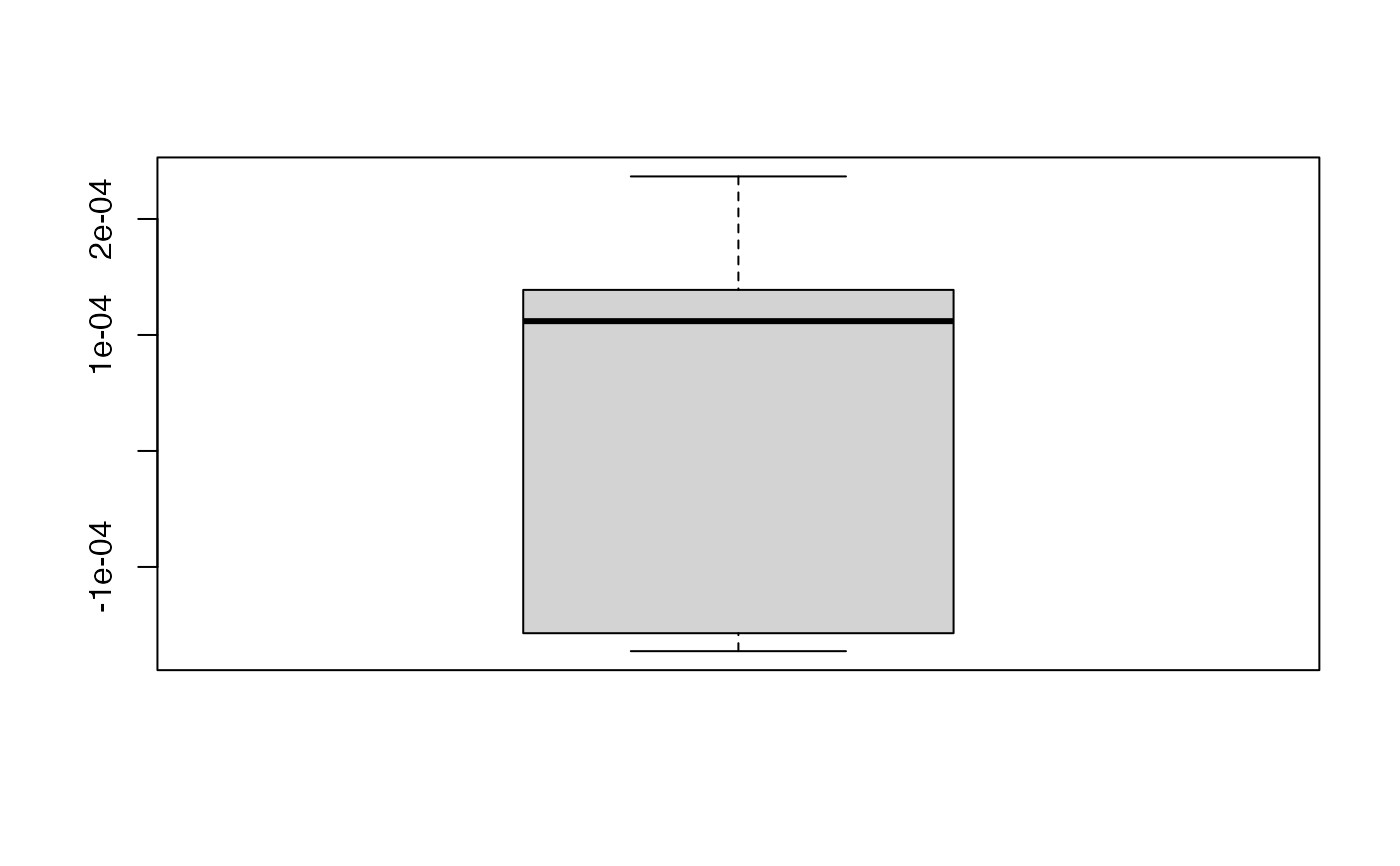 kfolds2Chisqind(bbb2)
#> [[1]]
#> [[1]][[1]]
#> [1] NA NA NA NA NA
#>
#> [[1]][[2]]
#> [1] NA NA NA NA NA NA
#>
#> [[1]][[3]]
#> [1] NA NA NA NA NA NA
#>
#> [[1]][[4]]
#> [1] NA NA NA NA NA NA
#>
#> [[1]][[5]]
#> [1] NA NA NA NA NA NA
#>
#>
kfolds2Chisq(bbb2)
#> [[1]]
#> [1] NA NA NA NA NA
#>
summary(bbb2)
#> ____************************************************____
#>
#> Family: inverse.gaussian
#> Link function: 1/mu^2
#>
#> ____Component____ 1 ____
#> ____Component____ 2 ____
#> ____Component____ 3 ____
#> ____Component____ 4 ____
#> ____Component____ 5 ____
#> ____Component____ 6 ____
#> ____Predicting X without NA neither in X or Y____
#> ****________________________________________________****
#>
#>
#> NK: 1
#> [[1]]
#> AIC BIC Q2Chisqcum_Y limQ2 Q2Chisq_Y PREChi2_Pearson_Y
#> Nb_Comp_0 81.67928 82.64909 NA NA NA NA
#> Nb_Comp_1 49.90521 51.35993 NA 0.0975 NA NA
#> Nb_Comp_2 31.06918 33.00881 NA 0.0975 NA NA
#> Nb_Comp_3 28.40632 30.83085 NA 0.0975 NA NA
#> Nb_Comp_4 27.08522 29.99466 NA 0.0975 NA NA
#> Nb_Comp_5 28.46056 31.85490 NA 0.0975 NA NA
#> Nb_Comp_6 29.68366 33.56292 NA 0.0975 NA NA
#> Chi2_Pearson_Y RSS_Y R2_Y
#> Nb_Comp_0 6.729783e-04 467.796667 NA
#> Nb_Comp_1 3.957680e-05 32.478677 0.9305710
#> Nb_Comp_2 7.009452e-06 6.020269 0.9871306
#> Nb_Comp_3 4.727777e-06 3.795855 0.9918857
#> Nb_Comp_4 3.584346e-06 2.699884 0.9942285
#> Nb_Comp_5 3.408069e-06 2.598572 0.9944451
#> Nb_Comp_6 3.195402e-06 2.492371 0.9946721
#>
#> attr(,"class")
#> [1] "summary.cv.plsRglmmodel"
PLS_lm(yCornell,XCornell,10,typeVC="standard")$InfCrit
#> ____************************************************____
#> ____TypeVC____ standard ____
#> ____Component____ 1 ____
#> ____Component____ 2 ____
#> ____Component____ 3 ____
#> ____Component____ 4 ____
#> ____Component____ 5 ____
#> ____Component____ 6 ____
#> Warning : < 10^{-12}
#> Warning only 6 components could thus be extracted
#> ____Predicting X without NA neither in X nor in Y____
#> ****________________________________________________****
#>
#> AIC Q2cum_Y LimQ2_Y Q2_Y PRESS_Y RSS_Y R2_Y
#> Nb_Comp_0 82.01205 NA NA NA NA 467.796667 NA
#> Nb_Comp_1 53.15173 0.8966556 0.0975 0.89665563 48.344150 35.742486 0.9235940
#> Nb_Comp_2 41.08283 0.9175426 0.0975 0.20210989 28.518576 11.066606 0.9763431
#> Nb_Comp_3 32.06411 0.9399676 0.0975 0.27195907 8.056942 4.418081 0.9905556
#> Nb_Comp_4 33.76477 0.9197009 0.0975 -0.33759604 5.909608 4.309235 0.9907882
#> Nb_Comp_5 33.34373 0.9281373 0.0975 0.10506161 3.856500 3.521924 0.9924713
#> Nb_Comp_6 35.25533 0.9232562 0.0975 -0.06792167 3.761138 3.496074 0.9925265
#> R2_residY RSS_residY PRESS_residY Q2_residY LimQ2 Q2cum_residY
#> Nb_Comp_0 NA 11.00000000 NA NA NA NA
#> Nb_Comp_1 0.9235940 0.84046633 1.13678803 0.89665563 0.0975 0.8966556
#> Nb_Comp_2 0.9763431 0.26022559 0.67059977 0.20210989 0.0975 0.9175426
#> Nb_Comp_3 0.9905556 0.10388893 0.18945488 0.27195907 0.0975 0.9399676
#> Nb_Comp_4 0.9907882 0.10132947 0.13896142 -0.33759604 0.0975 0.9197009
#> Nb_Comp_5 0.9924713 0.08281624 0.09068364 0.10506161 0.0975 0.9281373
#> Nb_Comp_6 0.9925265 0.08220840 0.08844125 -0.06792167 0.0975 0.9232562
#> AIC.std DoF.dof sigmahat.dof AIC.dof BIC.dof GMDL.dof
#> Nb_Comp_0 37.010388 1.000000 6.5212706 46.0708838 47.7893514 27.59461
#> Nb_Comp_1 8.150064 2.740749 1.8665281 4.5699686 4.9558156 21.34020
#> Nb_Comp_2 -3.918831 5.085967 1.1825195 2.1075461 2.3949331 27.40202
#> Nb_Comp_3 -12.937550 5.121086 0.7488308 0.8467795 0.9628191 24.40842
#> Nb_Comp_4 -11.236891 5.103312 0.7387162 0.8232505 0.9357846 24.23105
#> Nb_Comp_5 -11.657929 6.006316 0.7096382 0.7976101 0.9198348 28.21184
#> Nb_Comp_6 -9.746328 7.000002 0.7633343 0.9711321 1.1359501 33.18347
#> DoF.naive sigmahat.naive AIC.naive BIC.naive GMDL.naive
#> Nb_Comp_0 1 6.5212706 46.0708838 47.7893514 27.59461
#> Nb_Comp_1 2 1.8905683 4.1699567 4.4588195 18.37545
#> Nb_Comp_2 3 1.1088836 1.5370286 1.6860917 17.71117
#> Nb_Comp_3 4 0.7431421 0.7363469 0.8256118 19.01033
#> Nb_Comp_4 5 0.7846050 0.8721072 0.9964867 24.16510
#> Nb_Comp_5 6 0.7661509 0.8804809 1.0227979 28.64206
#> Nb_Comp_6 7 0.8361907 1.1070902 1.3048716 33.63927
rm(list=c("XCornell","yCornell","bbb","bbb2"))
# }
data(Cornell)
bbb <- cv.plsRglm(Y~.,data=Cornell,nt=10,NK=1,modele="pls")
#>
#> Model: pls
#>
#> NK: 1
#> Number of groups : 5
#> 1
#> ____************************************************____
#>
#> Model: pls
#>
#> ____Predicting X without NA neither in X nor in Y____
#> ____Component____ 1 ____
#> ____Component____ 2 ____
#> ____Component____ 3 ____
#> ____Component____ 4 ____
#> ____Component____ 5 ____
#> ____Component____ 6 ____
#> Warning : < 10^{-12}
#> Warning only 6 components could thus be extracted
#> ****________________________________________________****
#>
#> 2
#> ____************************************************____
#>
#> Model: pls
#>
#> ____Predicting X without NA neither in X nor in Y____
#> ____Component____ 1 ____
#> ____Component____ 2 ____
#> ____Component____ 3 ____
#> ____Component____ 4 ____
#> ____Component____ 5 ____
#> ____Component____ 6 ____
#> Warning : < 10^{-12}
#> Warning only 6 components could thus be extracted
#> ****________________________________________________****
#>
#> 3
#> ____************************************************____
#>
#> Model: pls
#>
#> ____Predicting X without NA neither in X nor in Y____
#> ____Component____ 1 ____
#> ____Component____ 2 ____
#> ____Component____ 3 ____
#> ____Component____ 4 ____
#> ____Component____ 5 ____
#> Warning : < 10^{-12}
#> Warning only 5 components could thus be extracted
#> ****________________________________________________****
#>
#> 4
#> ____************************************************____
#>
#> Model: pls
#>
#> ____Predicting X without NA neither in X nor in Y____
#> ____Component____ 1 ____
#> ____Component____ 2 ____
#> ____Component____ 3 ____
#> ____Component____ 4 ____
#> ____Component____ 5 ____
#> ____Component____ 6 ____
#> Warning : < 10^{-12}
#> Warning only 6 components could thus be extracted
#> ****________________________________________________****
#>
#> 5
#> ____************************************************____
#>
#> Model: pls
#>
#> ____Predicting X without NA neither in X nor in Y____
#> ____Component____ 1 ____
#> ____Component____ 2 ____
#> ____Component____ 3 ____
#> ____Component____ 4 ____
#> ____Component____ 5 ____
#> ____Component____ 6 ____
#> Warning : < 10^{-12}
#> Warning only 6 components could thus be extracted
#> ****________________________________________________****
#>
summary(bbb)
#> ____************************************************____
#>
#> Model: pls
#>
#> ____Component____ 1 ____
#> ____Component____ 2 ____
#> ____Component____ 3 ____
#> ____Component____ 4 ____
#> ____Component____ 5 ____
#> ____Component____ 6 ____
#> ____Predicting X without NA neither in X or Y____
#> ****________________________________________________****
#>
#>
#> NK: 1
#> [[1]]
#> AIC Q2cum_Y LimQ2_Y Q2_Y PRESS_Y RSS_Y R2_Y
#> Nb_Comp_0 82.01205 NA NA NA NA 467.796667 NA
#> Nb_Comp_1 53.15173 0.8825364 0.0975 0.8825364 54.94910 35.742486 0.9235940
#> Nb_Comp_2 41.08283 0.8269042 0.0975 -0.4736115 52.67054 11.066606 0.9763431
#> Nb_Comp_3 32.06411 0.5775041 0.0975 -1.4408218 27.01161 4.418081 0.9905556
#> Nb_Comp_4 33.76477 -0.6610330 0.0975 -2.9314767 17.36958 4.309235 0.9907882
#> Nb_Comp_5 33.34373 -4.2608140 0.0975 -2.1671942 13.64819 3.521924 0.9924713
#> Nb_Comp_6 35.25533 NA 0.0975 NA NA 3.496074 0.9925265
#> AIC.std DoF.dof sigmahat.dof AIC.dof BIC.dof GMDL.dof
#> Nb_Comp_0 37.010388 1.000000 6.5212706 46.0708838 47.7893514 27.59461
#> Nb_Comp_1 8.150064 2.740749 1.8665281 4.5699686 4.9558156 21.34020
#> Nb_Comp_2 -3.918831 5.085967 1.1825195 2.1075461 2.3949331 27.40202
#> Nb_Comp_3 -12.937550 5.121086 0.7488308 0.8467795 0.9628191 24.40842
#> Nb_Comp_4 -11.236891 5.103312 0.7387162 0.8232505 0.9357846 24.23105
#> Nb_Comp_5 -11.657929 6.006316 0.7096382 0.7976101 0.9198348 28.21184
#> Nb_Comp_6 -9.746328 7.000002 0.7633343 0.9711321 1.1359501 33.18347
#> DoF.naive sigmahat.naive AIC.naive BIC.naive GMDL.naive
#> Nb_Comp_0 1 6.5212706 46.0708838 47.7893514 27.59461
#> Nb_Comp_1 2 1.8905683 4.1699567 4.4588195 18.37545
#> Nb_Comp_2 3 1.1088836 1.5370286 1.6860917 17.71117
#> Nb_Comp_3 4 0.7431421 0.7363469 0.8256118 19.01033
#> Nb_Comp_4 5 0.7846050 0.8721072 0.9964867 24.16510
#> Nb_Comp_5 6 0.7661509 0.8804809 1.0227979 28.64206
#> Nb_Comp_6 7 0.8361907 1.1070902 1.3048716 33.63927
#>
#> attr(,"class")
#> [1] "summary.cv.plsRmodel"
cv.plsRglm(Y~.,data=Cornell,nt=3,modele="pls-glm-family",family=gaussian(),K=12)
#>
#> Family: gaussian
#> Link function: identity
#>
#> NK: 1
#> Leave One Out
#> Number of groups : 12
#> 1
#> ____************************************************____
#>
#> Family: gaussian
#> Link function: identity
#>
#> ____Predicting X without NA neither in X nor in Y____
#> ____Component____ 1 ____
#> ____Component____ 2 ____
#> ____Component____ 3 ____
#> ****________________________________________________****
#>
#> 2
#> ____************************************************____
#>
#> Family: gaussian
#> Link function: identity
#>
#> ____Predicting X without NA neither in X nor in Y____
#> ____Component____ 1 ____
#> ____Component____ 2 ____
#> ____Component____ 3 ____
#> ****________________________________________________****
#>
#> 3
#> ____************************************************____
#>
#> Family: gaussian
#> Link function: identity
#>
#> ____Predicting X without NA neither in X nor in Y____
#> ____Component____ 1 ____
#> ____Component____ 2 ____
#> ____Component____ 3 ____
#> ****________________________________________________****
#>
#> 4
#> ____************************************************____
#>
#> Family: gaussian
#> Link function: identity
#>
#> ____Predicting X without NA neither in X nor in Y____
#> ____Component____ 1 ____
#> ____Component____ 2 ____
#> ____Component____ 3 ____
#> ****________________________________________________****
#>
#> 5
#> ____************************************************____
#>
#> Family: gaussian
#> Link function: identity
#>
#> ____Predicting X without NA neither in X nor in Y____
#> ____Component____ 1 ____
#> ____Component____ 2 ____
#> ____Component____ 3 ____
#> ****________________________________________________****
#>
#> 6
#> ____************************************************____
#>
#> Family: gaussian
#> Link function: identity
#>
#> ____Predicting X without NA neither in X nor in Y____
#> ____Component____ 1 ____
#> ____Component____ 2 ____
#> ____Component____ 3 ____
#> ****________________________________________________****
#>
#> 7
#> ____************************************************____
#>
#> Family: gaussian
#> Link function: identity
#>
#> ____Predicting X without NA neither in X nor in Y____
#> ____Component____ 1 ____
#> ____Component____ 2 ____
#> ____Component____ 3 ____
#> ****________________________________________________****
#>
#> 8
#> ____************************************************____
#>
#> Family: gaussian
#> Link function: identity
#>
#> ____Predicting X without NA neither in X nor in Y____
#> ____Component____ 1 ____
#> ____Component____ 2 ____
#> ____Component____ 3 ____
#> ****________________________________________________****
#>
#> 9
#> ____************************************************____
#>
#> Family: gaussian
#> Link function: identity
#>
#> ____Predicting X without NA neither in X nor in Y____
#> ____Component____ 1 ____
#> ____Component____ 2 ____
#> ____Component____ 3 ____
#> ****________________________________________________****
#>
#> 10
#> ____************************************************____
#>
#> Family: gaussian
#> Link function: identity
#>
#> ____Predicting X without NA neither in X nor in Y____
#> ____Component____ 1 ____
#> ____Component____ 2 ____
#> ____Component____ 3 ____
#> ****________________________________________________****
#>
#> 11
#> ____************************************************____
#>
#> Family: gaussian
#> Link function: identity
#>
#> ____Predicting X without NA neither in X nor in Y____
#> ____Component____ 1 ____
#> ____Component____ 2 ____
#> ____Component____ 3 ____
#> ****________________________________________________****
#>
#> 12
#> ____************************************************____
#>
#> Family: gaussian
#> Link function: identity
#>
#> ____Predicting X without NA neither in X nor in Y____
#> ____Component____ 1 ____
#> ____Component____ 2 ____
#> ____Component____ 3 ____
#> ****________________________________________________****
#>
#> Number of repeated crossvalidations:
#> [1] 1
#> Number of folds for each crossvalidation:
#> [1] 12
# \donttest{
cv.plsRglm(Y~.,data=Cornell,nt=3,modele="pls-glm-family",family=gaussian(),K=6,
NK=2,random=TRUE,keepfolds=TRUE,verbose=FALSE)$results_kfolds
#> [[1]]
#> [[1]][[1]]
#> [,1] [,2] [,3]
#> 8 NA NA NA
#> 1 NA NA NA
#>
#> [[1]][[2]]
#> [,1] [,2] [,3]
#> 12 NA NA NA
#> 7 NA NA NA
#>
#> [[1]][[3]]
#> [,1] [,2] [,3]
#> 5 NA NA NA
#> 9 NA NA NA
#>
#> [[1]][[4]]
#> [,1] [,2] [,3]
#> 2 NA NA NA
#> 3 NA NA NA
#>
#> [[1]][[5]]
#> [,1] [,2] [,3]
#> 10 NA NA NA
#> 6 NA NA NA
#>
#> [[1]][[6]]
#> [,1] [,2] [,3]
#> 4 NA NA NA
#> 11 NA NA NA
#>
#>
#> [[2]]
#> [[2]][[1]]
#> [,1] [,2] [,3]
#> 1 NA NA NA
#> 8 NA NA NA
#>
#> [[2]][[2]]
#> [,1] [,2] [,3]
#> 9 NA NA NA
#> 10 NA NA NA
#>
#> [[2]][[3]]
#> [,1] [,2] [,3]
#> 2 NA NA NA
#> 7 NA NA NA
#>
#> [[2]][[4]]
#> [,1] [,2] [,3]
#> 11 NA NA NA
#> 5 NA NA NA
#>
#> [[2]][[5]]
#> [,1] [,2] [,3]
#> 12 NA NA NA
#> 4 NA NA NA
#>
#> [[2]][[6]]
#> [,1] [,2] [,3]
#> 6 NA NA NA
#> 3 NA NA NA
#>
#>
#Different ways of model specifications
cv.plsRglm(Y~.,data=Cornell,nt=3,modele="pls-glm-family",family=gaussian(),K=6,
NK=2,verbose=FALSE)$results_kfolds
#> [[1]]
#> [[1]][[1]]
#> [,1] [,2] [,3]
#> 3 NA NA NA
#> 6 NA NA NA
#>
#> [[1]][[2]]
#> [,1] [,2] [,3]
#> 7 NA NA NA
#> 2 NA NA NA
#>
#> [[1]][[3]]
#> [,1] [,2] [,3]
#> 1 NA NA NA
#> 4 NA NA NA
#>
#> [[1]][[4]]
#> [,1] [,2] [,3]
#> 5 NA NA NA
#> 8 NA NA NA
#>
#> [[1]][[5]]
#> [,1] [,2] [,3]
#> 10 NA NA NA
#> 12 NA NA NA
#>
#> [[1]][[6]]
#> [,1] [,2] [,3]
#> 11 NA NA NA
#> 9 NA NA NA
#>
#>
#> [[2]]
#> [[2]][[1]]
#> [,1] [,2] [,3]
#> 9 NA NA NA
#> 8 NA NA NA
#>
#> [[2]][[2]]
#> [,1] [,2] [,3]
#> 3 NA NA NA
#> 5 NA NA NA
#>
#> [[2]][[3]]
#> [,1] [,2] [,3]
#> 4 NA NA NA
#> 10 NA NA NA
#>
#> [[2]][[4]]
#> [,1] [,2] [,3]
#> 1 NA NA NA
#> 6 NA NA NA
#>
#> [[2]][[5]]
#> [,1] [,2] [,3]
#> 11 NA NA NA
#> 2 NA NA NA
#>
#> [[2]][[6]]
#> [,1] [,2] [,3]
#> 7 NA NA NA
#> 12 NA NA NA
#>
#>
cv.plsRglm(Y~.,data=Cornell,nt=3,modele="pls-glm-family",family=gaussian,
K=6,NK=2,verbose=FALSE)$results_kfolds
#> [[1]]
#> [[1]][[1]]
#> [,1] [,2] [,3]
#> 6 NA NA NA
#> 2 NA NA NA
#>
#> [[1]][[2]]
#> [,1] [,2] [,3]
#> 12 NA NA NA
#> 3 NA NA NA
#>
#> [[1]][[3]]
#> [,1] [,2] [,3]
#> 8 NA NA NA
#> 11 NA NA NA
#>
#> [[1]][[4]]
#> [,1] [,2] [,3]
#> 5 NA NA NA
#> 9 NA NA NA
#>
#> [[1]][[5]]
#> [,1] [,2] [,3]
#> 7 NA NA NA
#> 10 NA NA NA
#>
#> [[1]][[6]]
#> [,1] [,2] [,3]
#> 4 NA NA NA
#> 1 NA NA NA
#>
#>
#> [[2]]
#> [[2]][[1]]
#> [,1] [,2] [,3]
#> 8 NA NA NA
#> 6 NA NA NA
#>
#> [[2]][[2]]
#> [,1] [,2] [,3]
#> 11 NA NA NA
#> 12 NA NA NA
#>
#> [[2]][[3]]
#> [,1] [,2] [,3]
#> 9 NA NA NA
#> 1 NA NA NA
#>
#> [[2]][[4]]
#> [,1] [,2] [,3]
#> 2 NA NA NA
#> 7 NA NA NA
#>
#> [[2]][[5]]
#> [,1] [,2] [,3]
#> 4 NA NA NA
#> 5 NA NA NA
#>
#> [[2]][[6]]
#> [,1] [,2] [,3]
#> 10 NA NA NA
#> 3 NA NA NA
#>
#>
cv.plsRglm(Y~.,data=Cornell,nt=3,modele="pls-glm-family",family=gaussian(),
K=6,NK=2,verbose=FALSE)$results_kfolds
#> [[1]]
#> [[1]][[1]]
#> [,1] [,2] [,3]
#> 7 NA NA NA
#> 5 NA NA NA
#>
#> [[1]][[2]]
#> [,1] [,2] [,3]
#> 12 NA NA NA
#> 8 NA NA NA
#>
#> [[1]][[3]]
#> [,1] [,2] [,3]
#> 2 NA NA NA
#> 6 NA NA NA
#>
#> [[1]][[4]]
#> [,1] [,2] [,3]
#> 9 NA NA NA
#> 11 NA NA NA
#>
#> [[1]][[5]]
#> [,1] [,2] [,3]
#> 10 NA NA NA
#> 4 NA NA NA
#>
#> [[1]][[6]]
#> [,1] [,2] [,3]
#> 3 NA NA NA
#> 1 NA NA NA
#>
#>
#> [[2]]
#> [[2]][[1]]
#> [,1] [,2] [,3]
#> 10 NA NA NA
#> 2 NA NA NA
#>
#> [[2]][[2]]
#> [,1] [,2] [,3]
#> 7 NA NA NA
#> 6 NA NA NA
#>
#> [[2]][[3]]
#> [,1] [,2] [,3]
#> 3 NA NA NA
#> 5 NA NA NA
#>
#> [[2]][[4]]
#> [,1] [,2] [,3]
#> 11 NA NA NA
#> 8 NA NA NA
#>
#> [[2]][[5]]
#> [,1] [,2] [,3]
#> 12 NA NA NA
#> 9 NA NA NA
#>
#> [[2]][[6]]
#> [,1] [,2] [,3]
#> 4 NA NA NA
#> 1 NA NA NA
#>
#>
cv.plsRglm(Y~.,data=Cornell,nt=3,modele="pls-glm-family",family=gaussian(link=log),
K=6,NK=2,verbose=FALSE)$results_kfolds
#> [[1]]
#> [[1]][[1]]
#> [,1] [,2] [,3]
#> 3 NA NA NA
#> 5 NA NA NA
#>
#> [[1]][[2]]
#> [,1] [,2] [,3]
#> 4 NA NA NA
#> 6 NA NA NA
#>
#> [[1]][[3]]
#> [,1] [,2] [,3]
#> 7 NA NA NA
#> 2 NA NA NA
#>
#> [[1]][[4]]
#> [,1] [,2] [,3]
#> 9 NA NA NA
#> 12 NA NA NA
#>
#> [[1]][[5]]
#> [,1] [,2] [,3]
#> 11 NA NA NA
#> 1 NA NA NA
#>
#> [[1]][[6]]
#> [,1] [,2] [,3]
#> 8 NA NA NA
#> 10 NA NA NA
#>
#>
#> [[2]]
#> [[2]][[1]]
#> [,1] [,2] [,3]
#> 3 NA NA NA
#> 5 NA NA NA
#>
#> [[2]][[2]]
#> [,1] [,2] [,3]
#> 10 NA NA NA
#> 1 NA NA NA
#>
#> [[2]][[3]]
#> [,1] [,2] [,3]
#> 6 NA NA NA
#> 12 NA NA NA
#>
#> [[2]][[4]]
#> [,1] [,2] [,3]
#> 4 NA NA NA
#> 9 NA NA NA
#>
#> [[2]][[5]]
#> [,1] [,2] [,3]
#> 8 NA NA NA
#> 11 NA NA NA
#>
#> [[2]][[6]]
#> [,1] [,2] [,3]
#> 7 NA NA NA
#> 2 NA NA NA
#>
#>
bbb2 <- cv.plsRglm(Y~.,data=Cornell,nt=10,
modele="pls-glm-gaussian",keepcoeffs=TRUE,verbose=FALSE)
bbb2 <- cv.plsRglm(Y~.,data=Cornell,nt=3,modele="pls-glm-family",
family=gaussian(link=log),K=6,keepcoeffs=TRUE,verbose=FALSE)
#For Jackknife computations
kfolds2coeff(bbb2)
#> [,1] [,2] [,3] [,4] [,5] [,6]
#> [1,] 4.470273 -0.06317216 -0.015130085 -0.10739267 -0.05657930 0.030866914
#> [2,] 4.468766 -0.08427095 -0.019204062 -0.13596596 -0.05734367 0.031006389
#> [3,] 4.465960 -0.06389364 -0.019541280 -0.10394949 -0.05167567 0.060119790
#> [4,] 4.477324 -0.09243744 -0.027226841 -0.15458083 -0.05247624 0.022959125
#> [5,] 4.452397 -0.04645103 -0.004221374 -0.07332015 -0.04885178 -0.001590875
#> [6,] 4.496170 -0.08978082 -0.046226381 -0.14905411 -0.05666651 0.079637184
#> [,7] [,8]
#> [1,] 0.1612710 -0.2068408
#> [2,] 0.1628564 -0.1304898
#> [3,] 0.1729426 -0.2247461
#> [4,] 0.1554308 -0.2314175
#> [5,] 0.1889002 -0.2092133
#> [6,] 0.1230279 -0.3766808
boxplot(kfolds2coeff(bbb2)[,1])
kfolds2Chisqind(bbb2)
#> [[1]]
#> [[1]][[1]]
#> [1] NA NA NA NA NA
#>
#> [[1]][[2]]
#> [1] NA NA NA NA NA NA
#>
#> [[1]][[3]]
#> [1] NA NA NA NA NA NA
#>
#> [[1]][[4]]
#> [1] NA NA NA NA NA NA
#>
#> [[1]][[5]]
#> [1] NA NA NA NA NA NA
#>
#>
kfolds2Chisq(bbb2)
#> [[1]]
#> [1] NA NA NA NA NA
#>
summary(bbb2)
#> ____************************************************____
#>
#> Family: inverse.gaussian
#> Link function: 1/mu^2
#>
#> ____Component____ 1 ____
#> ____Component____ 2 ____
#> ____Component____ 3 ____
#> ____Component____ 4 ____
#> ____Component____ 5 ____
#> ____Component____ 6 ____
#> ____Predicting X without NA neither in X or Y____
#> ****________________________________________________****
#>
#>
#> NK: 1
#> [[1]]
#> AIC BIC Q2Chisqcum_Y limQ2 Q2Chisq_Y PREChi2_Pearson_Y
#> Nb_Comp_0 81.67928 82.64909 NA NA NA NA
#> Nb_Comp_1 49.90521 51.35993 NA 0.0975 NA NA
#> Nb_Comp_2 31.06918 33.00881 NA 0.0975 NA NA
#> Nb_Comp_3 28.40632 30.83085 NA 0.0975 NA NA
#> Nb_Comp_4 27.08522 29.99466 NA 0.0975 NA NA
#> Nb_Comp_5 28.46056 31.85490 NA 0.0975 NA NA
#> Nb_Comp_6 29.68366 33.56292 NA 0.0975 NA NA
#> Chi2_Pearson_Y RSS_Y R2_Y
#> Nb_Comp_0 6.729783e-04 467.796667 NA
#> Nb_Comp_1 3.957680e-05 32.478677 0.9305710
#> Nb_Comp_2 7.009452e-06 6.020269 0.9871306
#> Nb_Comp_3 4.727777e-06 3.795855 0.9918857
#> Nb_Comp_4 3.584346e-06 2.699884 0.9942285
#> Nb_Comp_5 3.408069e-06 2.598572 0.9944451
#> Nb_Comp_6 3.195402e-06 2.492371 0.9946721
#>
#> attr(,"class")
#> [1] "summary.cv.plsRglmmodel"
PLS_lm(yCornell,XCornell,10,typeVC="standard")$InfCrit
#> ____************************************************____
#> ____TypeVC____ standard ____
#> ____Component____ 1 ____
#> ____Component____ 2 ____
#> ____Component____ 3 ____
#> ____Component____ 4 ____
#> ____Component____ 5 ____
#> ____Component____ 6 ____
#> Warning : < 10^{-12}
#> Warning only 6 components could thus be extracted
#> ____Predicting X without NA neither in X nor in Y____
#> ****________________________________________________****
#>
#> AIC Q2cum_Y LimQ2_Y Q2_Y PRESS_Y RSS_Y R2_Y
#> Nb_Comp_0 82.01205 NA NA NA NA 467.796667 NA
#> Nb_Comp_1 53.15173 0.8966556 0.0975 0.89665563 48.344150 35.742486 0.9235940
#> Nb_Comp_2 41.08283 0.9175426 0.0975 0.20210989 28.518576 11.066606 0.9763431
#> Nb_Comp_3 32.06411 0.9399676 0.0975 0.27195907 8.056942 4.418081 0.9905556
#> Nb_Comp_4 33.76477 0.9197009 0.0975 -0.33759604 5.909608 4.309235 0.9907882
#> Nb_Comp_5 33.34373 0.9281373 0.0975 0.10506161 3.856500 3.521924 0.9924713
#> Nb_Comp_6 35.25533 0.9232562 0.0975 -0.06792167 3.761138 3.496074 0.9925265
#> R2_residY RSS_residY PRESS_residY Q2_residY LimQ2 Q2cum_residY
#> Nb_Comp_0 NA 11.00000000 NA NA NA NA
#> Nb_Comp_1 0.9235940 0.84046633 1.13678803 0.89665563 0.0975 0.8966556
#> Nb_Comp_2 0.9763431 0.26022559 0.67059977 0.20210989 0.0975 0.9175426
#> Nb_Comp_3 0.9905556 0.10388893 0.18945488 0.27195907 0.0975 0.9399676
#> Nb_Comp_4 0.9907882 0.10132947 0.13896142 -0.33759604 0.0975 0.9197009
#> Nb_Comp_5 0.9924713 0.08281624 0.09068364 0.10506161 0.0975 0.9281373
#> Nb_Comp_6 0.9925265 0.08220840 0.08844125 -0.06792167 0.0975 0.9232562
#> AIC.std DoF.dof sigmahat.dof AIC.dof BIC.dof GMDL.dof
#> Nb_Comp_0 37.010388 1.000000 6.5212706 46.0708838 47.7893514 27.59461
#> Nb_Comp_1 8.150064 2.740749 1.8665281 4.5699686 4.9558156 21.34020
#> Nb_Comp_2 -3.918831 5.085967 1.1825195 2.1075461 2.3949331 27.40202
#> Nb_Comp_3 -12.937550 5.121086 0.7488308 0.8467795 0.9628191 24.40842
#> Nb_Comp_4 -11.236891 5.103312 0.7387162 0.8232505 0.9357846 24.23105
#> Nb_Comp_5 -11.657929 6.006316 0.7096382 0.7976101 0.9198348 28.21184
#> Nb_Comp_6 -9.746328 7.000002 0.7633343 0.9711321 1.1359501 33.18347
#> DoF.naive sigmahat.naive AIC.naive BIC.naive GMDL.naive
#> Nb_Comp_0 1 6.5212706 46.0708838 47.7893514 27.59461
#> Nb_Comp_1 2 1.8905683 4.1699567 4.4588195 18.37545
#> Nb_Comp_2 3 1.1088836 1.5370286 1.6860917 17.71117
#> Nb_Comp_3 4 0.7431421 0.7363469 0.8256118 19.01033
#> Nb_Comp_4 5 0.7846050 0.8721072 0.9964867 24.16510
#> Nb_Comp_5 6 0.7661509 0.8804809 1.0227979 28.64206
#> Nb_Comp_6 7 0.8361907 1.1070902 1.3048716 33.63927
rm(list=c("XCornell","yCornell","bbb","bbb2"))
# }
data(Cornell)
bbb <- cv.plsRglm(Y~.,data=Cornell,nt=10,NK=1,modele="pls")
#>
#> Model: pls
#>
#> NK: 1
#> Number of groups : 5
#> 1
#> ____************************************************____
#>
#> Model: pls
#>
#> ____Predicting X without NA neither in X nor in Y____
#> ____Component____ 1 ____
#> ____Component____ 2 ____
#> ____Component____ 3 ____
#> ____Component____ 4 ____
#> ____Component____ 5 ____
#> ____Component____ 6 ____
#> Warning : < 10^{-12}
#> Warning only 6 components could thus be extracted
#> ****________________________________________________****
#>
#> 2
#> ____************************************************____
#>
#> Model: pls
#>
#> ____Predicting X without NA neither in X nor in Y____
#> ____Component____ 1 ____
#> ____Component____ 2 ____
#> ____Component____ 3 ____
#> ____Component____ 4 ____
#> ____Component____ 5 ____
#> ____Component____ 6 ____
#> Warning : < 10^{-12}
#> Warning only 6 components could thus be extracted
#> ****________________________________________________****
#>
#> 3
#> ____************************************************____
#>
#> Model: pls
#>
#> ____Predicting X without NA neither in X nor in Y____
#> ____Component____ 1 ____
#> ____Component____ 2 ____
#> ____Component____ 3 ____
#> ____Component____ 4 ____
#> ____Component____ 5 ____
#> Warning : < 10^{-12}
#> Warning only 5 components could thus be extracted
#> ****________________________________________________****
#>
#> 4
#> ____************************************************____
#>
#> Model: pls
#>
#> ____Predicting X without NA neither in X nor in Y____
#> ____Component____ 1 ____
#> ____Component____ 2 ____
#> ____Component____ 3 ____
#> ____Component____ 4 ____
#> ____Component____ 5 ____
#> ____Component____ 6 ____
#> Warning : < 10^{-12}
#> Warning only 6 components could thus be extracted
#> ****________________________________________________****
#>
#> 5
#> ____************************************************____
#>
#> Model: pls
#>
#> ____Predicting X without NA neither in X nor in Y____
#> ____Component____ 1 ____
#> ____Component____ 2 ____
#> ____Component____ 3 ____
#> ____Component____ 4 ____
#> ____Component____ 5 ____
#> ____Component____ 6 ____
#> Warning : < 10^{-12}
#> Warning only 6 components could thus be extracted
#> ****________________________________________________****
#>
summary(bbb)
#> ____************************************************____
#>
#> Model: pls
#>
#> ____Component____ 1 ____
#> ____Component____ 2 ____
#> ____Component____ 3 ____
#> ____Component____ 4 ____
#> ____Component____ 5 ____
#> ____Component____ 6 ____
#> ____Predicting X without NA neither in X or Y____
#> ****________________________________________________****
#>
#>
#> NK: 1
#> [[1]]
#> AIC Q2cum_Y LimQ2_Y Q2_Y PRESS_Y RSS_Y R2_Y
#> Nb_Comp_0 82.01205 NA NA NA NA 467.796667 NA
#> Nb_Comp_1 53.15173 0.8825364 0.0975 0.8825364 54.94910 35.742486 0.9235940
#> Nb_Comp_2 41.08283 0.8269042 0.0975 -0.4736115 52.67054 11.066606 0.9763431
#> Nb_Comp_3 32.06411 0.5775041 0.0975 -1.4408218 27.01161 4.418081 0.9905556
#> Nb_Comp_4 33.76477 -0.6610330 0.0975 -2.9314767 17.36958 4.309235 0.9907882
#> Nb_Comp_5 33.34373 -4.2608140 0.0975 -2.1671942 13.64819 3.521924 0.9924713
#> Nb_Comp_6 35.25533 NA 0.0975 NA NA 3.496074 0.9925265
#> AIC.std DoF.dof sigmahat.dof AIC.dof BIC.dof GMDL.dof
#> Nb_Comp_0 37.010388 1.000000 6.5212706 46.0708838 47.7893514 27.59461
#> Nb_Comp_1 8.150064 2.740749 1.8665281 4.5699686 4.9558156 21.34020
#> Nb_Comp_2 -3.918831 5.085967 1.1825195 2.1075461 2.3949331 27.40202
#> Nb_Comp_3 -12.937550 5.121086 0.7488308 0.8467795 0.9628191 24.40842
#> Nb_Comp_4 -11.236891 5.103312 0.7387162 0.8232505 0.9357846 24.23105
#> Nb_Comp_5 -11.657929 6.006316 0.7096382 0.7976101 0.9198348 28.21184
#> Nb_Comp_6 -9.746328 7.000002 0.7633343 0.9711321 1.1359501 33.18347
#> DoF.naive sigmahat.naive AIC.naive BIC.naive GMDL.naive
#> Nb_Comp_0 1 6.5212706 46.0708838 47.7893514 27.59461
#> Nb_Comp_1 2 1.8905683 4.1699567 4.4588195 18.37545
#> Nb_Comp_2 3 1.1088836 1.5370286 1.6860917 17.71117
#> Nb_Comp_3 4 0.7431421 0.7363469 0.8256118 19.01033
#> Nb_Comp_4 5 0.7846050 0.8721072 0.9964867 24.16510
#> Nb_Comp_5 6 0.7661509 0.8804809 1.0227979 28.64206
#> Nb_Comp_6 7 0.8361907 1.1070902 1.3048716 33.63927
#>
#> attr(,"class")
#> [1] "summary.cv.plsRmodel"
cv.plsRglm(Y~.,data=Cornell,nt=3,modele="pls-glm-family",family=gaussian(),K=12)
#>
#> Family: gaussian
#> Link function: identity
#>
#> NK: 1
#> Leave One Out
#> Number of groups : 12
#> 1
#> ____************************************************____
#>
#> Family: gaussian
#> Link function: identity
#>
#> ____Predicting X without NA neither in X nor in Y____
#> ____Component____ 1 ____
#> ____Component____ 2 ____
#> ____Component____ 3 ____
#> ****________________________________________________****
#>
#> 2
#> ____************************************************____
#>
#> Family: gaussian
#> Link function: identity
#>
#> ____Predicting X without NA neither in X nor in Y____
#> ____Component____ 1 ____
#> ____Component____ 2 ____
#> ____Component____ 3 ____
#> ****________________________________________________****
#>
#> 3
#> ____************************************************____
#>
#> Family: gaussian
#> Link function: identity
#>
#> ____Predicting X without NA neither in X nor in Y____
#> ____Component____ 1 ____
#> ____Component____ 2 ____
#> ____Component____ 3 ____
#> ****________________________________________________****
#>
#> 4
#> ____************************************************____
#>
#> Family: gaussian
#> Link function: identity
#>
#> ____Predicting X without NA neither in X nor in Y____
#> ____Component____ 1 ____
#> ____Component____ 2 ____
#> ____Component____ 3 ____
#> ****________________________________________________****
#>
#> 5
#> ____************************************************____
#>
#> Family: gaussian
#> Link function: identity
#>
#> ____Predicting X without NA neither in X nor in Y____
#> ____Component____ 1 ____
#> ____Component____ 2 ____
#> ____Component____ 3 ____
#> ****________________________________________________****
#>
#> 6
#> ____************************************************____
#>
#> Family: gaussian
#> Link function: identity
#>
#> ____Predicting X without NA neither in X nor in Y____
#> ____Component____ 1 ____
#> ____Component____ 2 ____
#> ____Component____ 3 ____
#> ****________________________________________________****
#>
#> 7
#> ____************************************************____
#>
#> Family: gaussian
#> Link function: identity
#>
#> ____Predicting X without NA neither in X nor in Y____
#> ____Component____ 1 ____
#> ____Component____ 2 ____
#> ____Component____ 3 ____
#> ****________________________________________________****
#>
#> 8
#> ____************************************************____
#>
#> Family: gaussian
#> Link function: identity
#>
#> ____Predicting X without NA neither in X nor in Y____
#> ____Component____ 1 ____
#> ____Component____ 2 ____
#> ____Component____ 3 ____
#> ****________________________________________________****
#>
#> 9
#> ____************************************************____
#>
#> Family: gaussian
#> Link function: identity
#>
#> ____Predicting X without NA neither in X nor in Y____
#> ____Component____ 1 ____
#> ____Component____ 2 ____
#> ____Component____ 3 ____
#> ****________________________________________________****
#>
#> 10
#> ____************************************************____
#>
#> Family: gaussian
#> Link function: identity
#>
#> ____Predicting X without NA neither in X nor in Y____
#> ____Component____ 1 ____
#> ____Component____ 2 ____
#> ____Component____ 3 ____
#> ****________________________________________________****
#>
#> 11
#> ____************************************************____
#>
#> Family: gaussian
#> Link function: identity
#>
#> ____Predicting X without NA neither in X nor in Y____
#> ____Component____ 1 ____
#> ____Component____ 2 ____
#> ____Component____ 3 ____
#> ****________________________________________________****
#>
#> 12
#> ____************************************************____
#>
#> Family: gaussian
#> Link function: identity
#>
#> ____Predicting X without NA neither in X nor in Y____
#> ____Component____ 1 ____
#> ____Component____ 2 ____
#> ____Component____ 3 ____
#> ****________________________________________________****
#>
#> Number of repeated crossvalidations:
#> [1] 1
#> Number of folds for each crossvalidation:
#> [1] 12
# \donttest{
cv.plsRglm(Y~.,data=Cornell,nt=3,modele="pls-glm-family",family=gaussian(),K=6,
NK=2,random=TRUE,keepfolds=TRUE,verbose=FALSE)$results_kfolds
#> [[1]]
#> [[1]][[1]]
#> [,1] [,2] [,3]
#> 8 NA NA NA
#> 1 NA NA NA
#>
#> [[1]][[2]]
#> [,1] [,2] [,3]
#> 12 NA NA NA
#> 7 NA NA NA
#>
#> [[1]][[3]]
#> [,1] [,2] [,3]
#> 5 NA NA NA
#> 9 NA NA NA
#>
#> [[1]][[4]]
#> [,1] [,2] [,3]
#> 2 NA NA NA
#> 3 NA NA NA
#>
#> [[1]][[5]]
#> [,1] [,2] [,3]
#> 10 NA NA NA
#> 6 NA NA NA
#>
#> [[1]][[6]]
#> [,1] [,2] [,3]
#> 4 NA NA NA
#> 11 NA NA NA
#>
#>
#> [[2]]
#> [[2]][[1]]
#> [,1] [,2] [,3]
#> 1 NA NA NA
#> 8 NA NA NA
#>
#> [[2]][[2]]
#> [,1] [,2] [,3]
#> 9 NA NA NA
#> 10 NA NA NA
#>
#> [[2]][[3]]
#> [,1] [,2] [,3]
#> 2 NA NA NA
#> 7 NA NA NA
#>
#> [[2]][[4]]
#> [,1] [,2] [,3]
#> 11 NA NA NA
#> 5 NA NA NA
#>
#> [[2]][[5]]
#> [,1] [,2] [,3]
#> 12 NA NA NA
#> 4 NA NA NA
#>
#> [[2]][[6]]
#> [,1] [,2] [,3]
#> 6 NA NA NA
#> 3 NA NA NA
#>
#>
#Different ways of model specifications
cv.plsRglm(Y~.,data=Cornell,nt=3,modele="pls-glm-family",family=gaussian(),K=6,
NK=2,verbose=FALSE)$results_kfolds
#> [[1]]
#> [[1]][[1]]
#> [,1] [,2] [,3]
#> 3 NA NA NA
#> 6 NA NA NA
#>
#> [[1]][[2]]
#> [,1] [,2] [,3]
#> 7 NA NA NA
#> 2 NA NA NA
#>
#> [[1]][[3]]
#> [,1] [,2] [,3]
#> 1 NA NA NA
#> 4 NA NA NA
#>
#> [[1]][[4]]
#> [,1] [,2] [,3]
#> 5 NA NA NA
#> 8 NA NA NA
#>
#> [[1]][[5]]
#> [,1] [,2] [,3]
#> 10 NA NA NA
#> 12 NA NA NA
#>
#> [[1]][[6]]
#> [,1] [,2] [,3]
#> 11 NA NA NA
#> 9 NA NA NA
#>
#>
#> [[2]]
#> [[2]][[1]]
#> [,1] [,2] [,3]
#> 9 NA NA NA
#> 8 NA NA NA
#>
#> [[2]][[2]]
#> [,1] [,2] [,3]
#> 3 NA NA NA
#> 5 NA NA NA
#>
#> [[2]][[3]]
#> [,1] [,2] [,3]
#> 4 NA NA NA
#> 10 NA NA NA
#>
#> [[2]][[4]]
#> [,1] [,2] [,3]
#> 1 NA NA NA
#> 6 NA NA NA
#>
#> [[2]][[5]]
#> [,1] [,2] [,3]
#> 11 NA NA NA
#> 2 NA NA NA
#>
#> [[2]][[6]]
#> [,1] [,2] [,3]
#> 7 NA NA NA
#> 12 NA NA NA
#>
#>
cv.plsRglm(Y~.,data=Cornell,nt=3,modele="pls-glm-family",family=gaussian,
K=6,NK=2,verbose=FALSE)$results_kfolds
#> [[1]]
#> [[1]][[1]]
#> [,1] [,2] [,3]
#> 6 NA NA NA
#> 2 NA NA NA
#>
#> [[1]][[2]]
#> [,1] [,2] [,3]
#> 12 NA NA NA
#> 3 NA NA NA
#>
#> [[1]][[3]]
#> [,1] [,2] [,3]
#> 8 NA NA NA
#> 11 NA NA NA
#>
#> [[1]][[4]]
#> [,1] [,2] [,3]
#> 5 NA NA NA
#> 9 NA NA NA
#>
#> [[1]][[5]]
#> [,1] [,2] [,3]
#> 7 NA NA NA
#> 10 NA NA NA
#>
#> [[1]][[6]]
#> [,1] [,2] [,3]
#> 4 NA NA NA
#> 1 NA NA NA
#>
#>
#> [[2]]
#> [[2]][[1]]
#> [,1] [,2] [,3]
#> 8 NA NA NA
#> 6 NA NA NA
#>
#> [[2]][[2]]
#> [,1] [,2] [,3]
#> 11 NA NA NA
#> 12 NA NA NA
#>
#> [[2]][[3]]
#> [,1] [,2] [,3]
#> 9 NA NA NA
#> 1 NA NA NA
#>
#> [[2]][[4]]
#> [,1] [,2] [,3]
#> 2 NA NA NA
#> 7 NA NA NA
#>
#> [[2]][[5]]
#> [,1] [,2] [,3]
#> 4 NA NA NA
#> 5 NA NA NA
#>
#> [[2]][[6]]
#> [,1] [,2] [,3]
#> 10 NA NA NA
#> 3 NA NA NA
#>
#>
cv.plsRglm(Y~.,data=Cornell,nt=3,modele="pls-glm-family",family=gaussian(),
K=6,NK=2,verbose=FALSE)$results_kfolds
#> [[1]]
#> [[1]][[1]]
#> [,1] [,2] [,3]
#> 7 NA NA NA
#> 5 NA NA NA
#>
#> [[1]][[2]]
#> [,1] [,2] [,3]
#> 12 NA NA NA
#> 8 NA NA NA
#>
#> [[1]][[3]]
#> [,1] [,2] [,3]
#> 2 NA NA NA
#> 6 NA NA NA
#>
#> [[1]][[4]]
#> [,1] [,2] [,3]
#> 9 NA NA NA
#> 11 NA NA NA
#>
#> [[1]][[5]]
#> [,1] [,2] [,3]
#> 10 NA NA NA
#> 4 NA NA NA
#>
#> [[1]][[6]]
#> [,1] [,2] [,3]
#> 3 NA NA NA
#> 1 NA NA NA
#>
#>
#> [[2]]
#> [[2]][[1]]
#> [,1] [,2] [,3]
#> 10 NA NA NA
#> 2 NA NA NA
#>
#> [[2]][[2]]
#> [,1] [,2] [,3]
#> 7 NA NA NA
#> 6 NA NA NA
#>
#> [[2]][[3]]
#> [,1] [,2] [,3]
#> 3 NA NA NA
#> 5 NA NA NA
#>
#> [[2]][[4]]
#> [,1] [,2] [,3]
#> 11 NA NA NA
#> 8 NA NA NA
#>
#> [[2]][[5]]
#> [,1] [,2] [,3]
#> 12 NA NA NA
#> 9 NA NA NA
#>
#> [[2]][[6]]
#> [,1] [,2] [,3]
#> 4 NA NA NA
#> 1 NA NA NA
#>
#>
cv.plsRglm(Y~.,data=Cornell,nt=3,modele="pls-glm-family",family=gaussian(link=log),
K=6,NK=2,verbose=FALSE)$results_kfolds
#> [[1]]
#> [[1]][[1]]
#> [,1] [,2] [,3]
#> 3 NA NA NA
#> 5 NA NA NA
#>
#> [[1]][[2]]
#> [,1] [,2] [,3]
#> 4 NA NA NA
#> 6 NA NA NA
#>
#> [[1]][[3]]
#> [,1] [,2] [,3]
#> 7 NA NA NA
#> 2 NA NA NA
#>
#> [[1]][[4]]
#> [,1] [,2] [,3]
#> 9 NA NA NA
#> 12 NA NA NA
#>
#> [[1]][[5]]
#> [,1] [,2] [,3]
#> 11 NA NA NA
#> 1 NA NA NA
#>
#> [[1]][[6]]
#> [,1] [,2] [,3]
#> 8 NA NA NA
#> 10 NA NA NA
#>
#>
#> [[2]]
#> [[2]][[1]]
#> [,1] [,2] [,3]
#> 3 NA NA NA
#> 5 NA NA NA
#>
#> [[2]][[2]]
#> [,1] [,2] [,3]
#> 10 NA NA NA
#> 1 NA NA NA
#>
#> [[2]][[3]]
#> [,1] [,2] [,3]
#> 6 NA NA NA
#> 12 NA NA NA
#>
#> [[2]][[4]]
#> [,1] [,2] [,3]
#> 4 NA NA NA
#> 9 NA NA NA
#>
#> [[2]][[5]]
#> [,1] [,2] [,3]
#> 8 NA NA NA
#> 11 NA NA NA
#>
#> [[2]][[6]]
#> [,1] [,2] [,3]
#> 7 NA NA NA
#> 2 NA NA NA
#>
#>
bbb2 <- cv.plsRglm(Y~.,data=Cornell,nt=10,
modele="pls-glm-gaussian",keepcoeffs=TRUE,verbose=FALSE)
bbb2 <- cv.plsRglm(Y~.,data=Cornell,nt=3,modele="pls-glm-family",
family=gaussian(link=log),K=6,keepcoeffs=TRUE,verbose=FALSE)
#For Jackknife computations
kfolds2coeff(bbb2)
#> [,1] [,2] [,3] [,4] [,5] [,6]
#> [1,] 4.470273 -0.06317216 -0.015130085 -0.10739267 -0.05657930 0.030866914
#> [2,] 4.468766 -0.08427095 -0.019204062 -0.13596596 -0.05734367 0.031006389
#> [3,] 4.465960 -0.06389364 -0.019541280 -0.10394949 -0.05167567 0.060119790
#> [4,] 4.477324 -0.09243744 -0.027226841 -0.15458083 -0.05247624 0.022959125
#> [5,] 4.452397 -0.04645103 -0.004221374 -0.07332015 -0.04885178 -0.001590875
#> [6,] 4.496170 -0.08978082 -0.046226381 -0.14905411 -0.05666651 0.079637184
#> [,7] [,8]
#> [1,] 0.1612710 -0.2068408
#> [2,] 0.1628564 -0.1304898
#> [3,] 0.1729426 -0.2247461
#> [4,] 0.1554308 -0.2314175
#> [5,] 0.1889002 -0.2092133
#> [6,] 0.1230279 -0.3766808
boxplot(kfolds2coeff(bbb2)[,1])
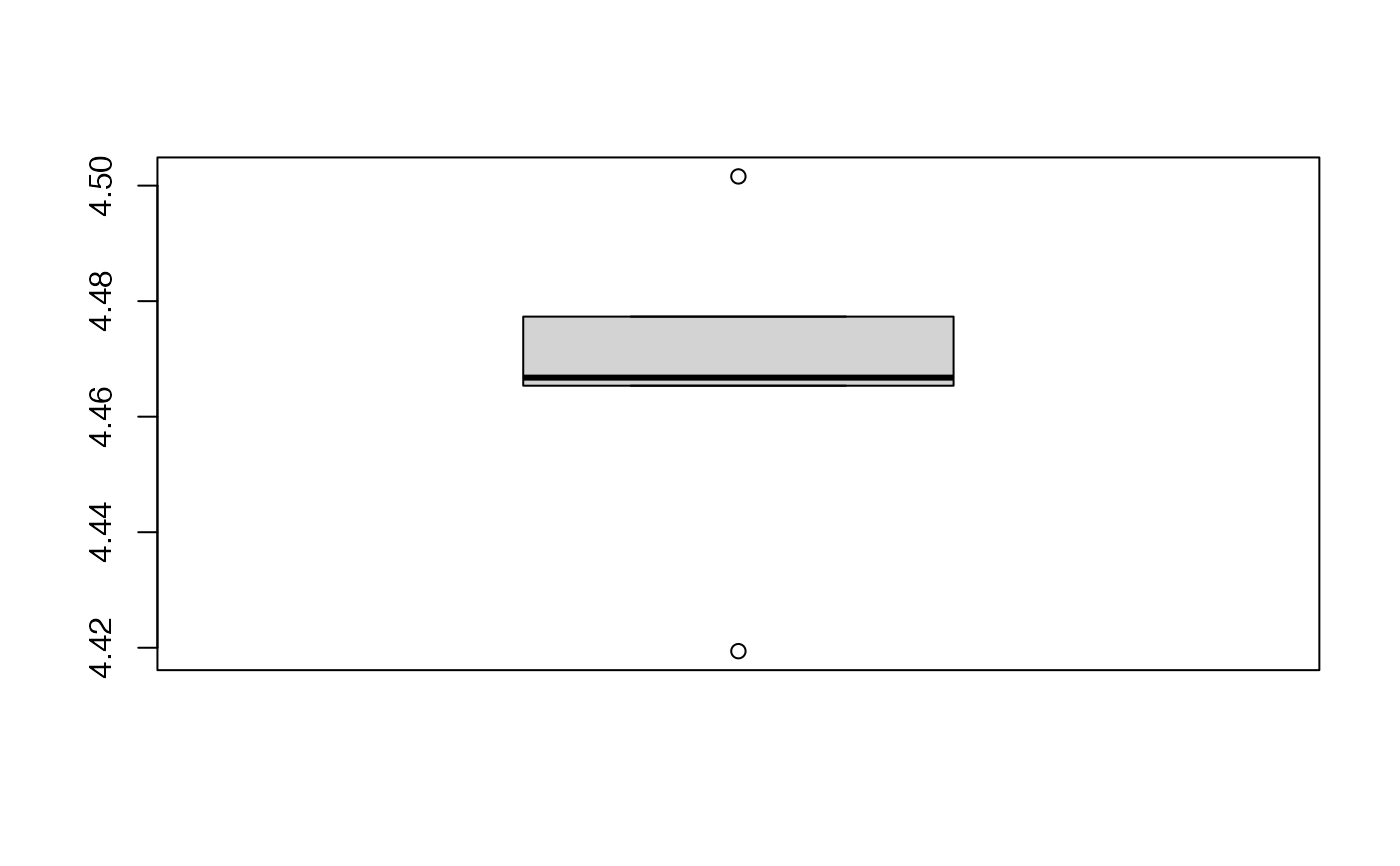 kfolds2Chisqind(bbb2)
#> [[1]]
#> [[1]][[1]]
#> [1] NA NA NA
#>
#> [[1]][[2]]
#> [1] NA NA NA
#>
#> [[1]][[3]]
#> [1] NA NA NA
#>
#> [[1]][[4]]
#> [1] NA NA NA
#>
#> [[1]][[5]]
#> [1] NA NA NA
#>
#> [[1]][[6]]
#> [1] NA NA NA
#>
#>
kfolds2Chisq(bbb2)
#> [[1]]
#> [1] NA NA NA
#>
summary(bbb2)
#> ____************************************************____
#>
#> Family: gaussian
#> Link function: log
#>
#> ____Component____ 1 ____
#> ____Component____ 2 ____
#> ____Component____ 3 ____
#> ____Predicting X without NA neither in X or Y____
#> ****________________________________________________****
#>
#>
#> NK: 1
#> [[1]]
#> AIC BIC Q2Chisqcum_Y limQ2 Q2Chisq_Y PREChi2_Pearson_Y
#> Nb_Comp_0 82.01205 82.98186 NA NA NA NA
#> Nb_Comp_1 52.67938 54.13410 NA 0.0975 NA NA
#> Nb_Comp_2 32.16524 34.10487 NA 0.0975 NA NA
#> Nb_Comp_3 30.58789 33.01242 NA 0.0975 NA NA
#> Chi2_Pearson_Y RSS_Y R2_Y
#> Nb_Comp_0 467.796667 467.796667 NA
#> Nb_Comp_1 34.362913 34.362913 0.9265431
#> Nb_Comp_2 5.263520 5.263520 0.9887483
#> Nb_Comp_3 3.906676 3.906676 0.9916488
#>
#> attr(,"class")
#> [1] "summary.cv.plsRglmmodel"
PLS_lm_formula(Y~.,data=Cornell,10,typeVC="standard")$InfCrit
#> ____************************************************____
#> ____TypeVC____ standard ____
#> ____Component____ 1 ____
#> ____Component____ 2 ____
#> ____Component____ 3 ____
#> ____Component____ 4 ____
#> ____Component____ 5 ____
#> ____Component____ 6 ____
#> Warning : 1 2 3 4 5 6 7 < 10^{-12}
#> Warning only 6 components could thus be extracted
#> ____Predicting X without NA neither in X nor in Y____
#> ****________________________________________________****
#>
#> AIC Q2cum_Y LimQ2_Y Q2_Y PRESS_Y RSS_Y R2_Y
#> Nb_Comp_0 82.01205 NA NA NA NA 467.796667 NA
#> Nb_Comp_1 53.15173 0.8966556 0.0975 0.89665563 48.344150 35.742486 0.9235940
#> Nb_Comp_2 41.08283 0.9175426 0.0975 0.20210989 28.518576 11.066606 0.9763431
#> Nb_Comp_3 32.06411 0.9399676 0.0975 0.27195907 8.056942 4.418081 0.9905556
#> Nb_Comp_4 33.76477 0.9197009 0.0975 -0.33759604 5.909608 4.309235 0.9907882
#> Nb_Comp_5 33.34373 0.9281373 0.0975 0.10506161 3.856500 3.521924 0.9924713
#> Nb_Comp_6 35.25533 0.9232562 0.0975 -0.06792167 3.761138 3.496074 0.9925265
#> R2_residY RSS_residY PRESS_residY Q2_residY LimQ2 Q2cum_residY
#> Nb_Comp_0 NA 11.00000000 NA NA NA NA
#> Nb_Comp_1 0.9235940 0.84046633 1.13678803 0.89665563 0.0975 0.8966556
#> Nb_Comp_2 0.9763431 0.26022559 0.67059977 0.20210989 0.0975 0.9175426
#> Nb_Comp_3 0.9905556 0.10388893 0.18945488 0.27195907 0.0975 0.9399676
#> Nb_Comp_4 0.9907882 0.10132947 0.13896142 -0.33759604 0.0975 0.9197009
#> Nb_Comp_5 0.9924713 0.08281624 0.09068364 0.10506161 0.0975 0.9281373
#> Nb_Comp_6 0.9925265 0.08220840 0.08844125 -0.06792167 0.0975 0.9232562
#> AIC.std DoF.dof sigmahat.dof AIC.dof BIC.dof GMDL.dof
#> Nb_Comp_0 37.010388 1.000000 6.5212706 46.0708838 47.7893514 27.59461
#> Nb_Comp_1 8.150064 2.740749 1.8665281 4.5699686 4.9558156 21.34020
#> Nb_Comp_2 -3.918831 5.085967 1.1825195 2.1075461 2.3949331 27.40202
#> Nb_Comp_3 -12.937550 5.121086 0.7488308 0.8467795 0.9628191 24.40842
#> Nb_Comp_4 -11.236891 5.103312 0.7387162 0.8232505 0.9357846 24.23105
#> Nb_Comp_5 -11.657929 6.006316 0.7096382 0.7976101 0.9198348 28.21184
#> Nb_Comp_6 -9.746328 7.000001 0.7633342 0.9711319 1.1359499 33.18347
#> DoF.naive sigmahat.naive AIC.naive BIC.naive GMDL.naive
#> Nb_Comp_0 1 6.5212706 46.0708838 47.7893514 27.59461
#> Nb_Comp_1 2 1.8905683 4.1699567 4.4588195 18.37545
#> Nb_Comp_2 3 1.1088836 1.5370286 1.6860917 17.71117
#> Nb_Comp_3 4 0.7431421 0.7363469 0.8256118 19.01033
#> Nb_Comp_4 5 0.7846050 0.8721072 0.9964867 24.16510
#> Nb_Comp_5 6 0.7661509 0.8804809 1.0227979 28.64206
#> Nb_Comp_6 7 0.8361907 1.1070902 1.3048716 33.63927
rm(list=c("bbb","bbb2"))
data(pine)
bbb <- cv.plsRglm(x11~.,data=pine,nt=10,modele="pls-glm-family",
family=gaussian(log),K=10,keepcoeffs=TRUE,keepfolds=FALSE,verbose=FALSE)
#> Warning: glm.fit: algorithm did not converge
#> Warning: glm.fit: algorithm did not converge
#> Warning: glm.fit: algorithm did not converge
#> Warning: glm.fit: algorithm did not converge
#> Warning: glm.fit: algorithm did not converge
#> Warning: glm.fit: algorithm did not converge
#> Warning: glm.fit: algorithm did not converge
#> Warning: glm.fit: algorithm did not converge
#> Warning: glm.fit: algorithm did not converge
#> Warning: glm.fit: algorithm did not converge
#> Warning: glm.fit: algorithm did not converge
#> Warning: glm.fit: algorithm did not converge
#> Warning: glm.fit: algorithm did not converge
#> Warning: glm.fit: algorithm did not converge
#> Warning: glm.fit: algorithm did not converge
#> Warning: glm.fit: algorithm did not converge
#> Warning: glm.fit: algorithm did not converge
bbb <- cv.plsRglm(x11~.,data=pine,nt=10,modele="pls-glm-family",family=gaussian(),
K=10,keepcoeffs=TRUE,keepfolds=FALSE,verbose=FALSE)
#For Jackknife computations
kfolds2coeff(bbb)
#> [,1] [,2] [,3] [,4] [,5] [,6]
#> [1,] 8.156030 -0.002843084 -0.03644892 0.027297442 -0.4943102 0.10194191
#> [2,] 8.588526 -0.002897746 -0.03843733 0.018948973 -0.5076750 0.10318074
#> [3,] 7.346555 -0.002639189 -0.03197018 0.029176977 -0.3788608 0.09274711
#> [4,] 7.644263 -0.002720788 -0.03020072 0.025195551 -0.5070876 0.11257349
#> [5,] 9.468184 -0.003056342 -0.03244721 0.080968844 -0.5349550 0.08134066
#> [6,] 8.476948 -0.003052482 -0.03844314 0.043200815 -0.3823907 0.09840346
#> [7,] 7.485734 -0.002118536 -0.03848000 0.006338868 -0.1314073 0.03168094
#> [8,] 8.415013 -0.003637688 -0.03532410 0.026646064 -0.6087039 0.17020306
#> [9,] 9.000407 -0.003254954 -0.03482172 0.027392108 -0.5920017 0.12489329
#> [10,] 8.641954 -0.002960673 -0.03038941 0.024750762 -0.4061744 0.09193541
#> [,7] [,8] [,9] [,10] [,11]
#> [1,] -0.02168238 -0.32787943 0.0522727243 -0.7800157 -0.268530683
#> [2,] 0.31824223 -0.41832606 0.0139150953 -0.8928500 -0.330604891
#> [3,] 0.09974150 0.02083909 0.0009329017 -0.8186071 -0.516438300
#> [4,] -0.01614965 -0.22930917 0.0376489360 -0.7629602 -0.294052133
#> [5,] -0.74630708 -0.22164995 0.1547819588 -1.1247555 -0.416971506
#> [6,] -0.21142520 -0.22984493 0.0096712788 -0.7951799 -0.316391684
#> [7,] 0.51108868 -0.64801419 -0.0627153804 -1.0417407 0.000622326
#> [8,] -0.06239897 0.12598389 -0.0484719959 -0.5177580 -0.379773648
#> [9,] 0.33490906 -0.45844428 0.0711930649 -1.2312607 -0.222402358
#> [10,] 0.18660012 -0.36608742 0.0016756723 -0.9511047 -0.435404655
boxplot(kfolds2coeff(bbb)[,1])
kfolds2Chisqind(bbb2)
#> [[1]]
#> [[1]][[1]]
#> [1] NA NA NA
#>
#> [[1]][[2]]
#> [1] NA NA NA
#>
#> [[1]][[3]]
#> [1] NA NA NA
#>
#> [[1]][[4]]
#> [1] NA NA NA
#>
#> [[1]][[5]]
#> [1] NA NA NA
#>
#> [[1]][[6]]
#> [1] NA NA NA
#>
#>
kfolds2Chisq(bbb2)
#> [[1]]
#> [1] NA NA NA
#>
summary(bbb2)
#> ____************************************************____
#>
#> Family: gaussian
#> Link function: log
#>
#> ____Component____ 1 ____
#> ____Component____ 2 ____
#> ____Component____ 3 ____
#> ____Predicting X without NA neither in X or Y____
#> ****________________________________________________****
#>
#>
#> NK: 1
#> [[1]]
#> AIC BIC Q2Chisqcum_Y limQ2 Q2Chisq_Y PREChi2_Pearson_Y
#> Nb_Comp_0 82.01205 82.98186 NA NA NA NA
#> Nb_Comp_1 52.67938 54.13410 NA 0.0975 NA NA
#> Nb_Comp_2 32.16524 34.10487 NA 0.0975 NA NA
#> Nb_Comp_3 30.58789 33.01242 NA 0.0975 NA NA
#> Chi2_Pearson_Y RSS_Y R2_Y
#> Nb_Comp_0 467.796667 467.796667 NA
#> Nb_Comp_1 34.362913 34.362913 0.9265431
#> Nb_Comp_2 5.263520 5.263520 0.9887483
#> Nb_Comp_3 3.906676 3.906676 0.9916488
#>
#> attr(,"class")
#> [1] "summary.cv.plsRglmmodel"
PLS_lm_formula(Y~.,data=Cornell,10,typeVC="standard")$InfCrit
#> ____************************************************____
#> ____TypeVC____ standard ____
#> ____Component____ 1 ____
#> ____Component____ 2 ____
#> ____Component____ 3 ____
#> ____Component____ 4 ____
#> ____Component____ 5 ____
#> ____Component____ 6 ____
#> Warning : 1 2 3 4 5 6 7 < 10^{-12}
#> Warning only 6 components could thus be extracted
#> ____Predicting X without NA neither in X nor in Y____
#> ****________________________________________________****
#>
#> AIC Q2cum_Y LimQ2_Y Q2_Y PRESS_Y RSS_Y R2_Y
#> Nb_Comp_0 82.01205 NA NA NA NA 467.796667 NA
#> Nb_Comp_1 53.15173 0.8966556 0.0975 0.89665563 48.344150 35.742486 0.9235940
#> Nb_Comp_2 41.08283 0.9175426 0.0975 0.20210989 28.518576 11.066606 0.9763431
#> Nb_Comp_3 32.06411 0.9399676 0.0975 0.27195907 8.056942 4.418081 0.9905556
#> Nb_Comp_4 33.76477 0.9197009 0.0975 -0.33759604 5.909608 4.309235 0.9907882
#> Nb_Comp_5 33.34373 0.9281373 0.0975 0.10506161 3.856500 3.521924 0.9924713
#> Nb_Comp_6 35.25533 0.9232562 0.0975 -0.06792167 3.761138 3.496074 0.9925265
#> R2_residY RSS_residY PRESS_residY Q2_residY LimQ2 Q2cum_residY
#> Nb_Comp_0 NA 11.00000000 NA NA NA NA
#> Nb_Comp_1 0.9235940 0.84046633 1.13678803 0.89665563 0.0975 0.8966556
#> Nb_Comp_2 0.9763431 0.26022559 0.67059977 0.20210989 0.0975 0.9175426
#> Nb_Comp_3 0.9905556 0.10388893 0.18945488 0.27195907 0.0975 0.9399676
#> Nb_Comp_4 0.9907882 0.10132947 0.13896142 -0.33759604 0.0975 0.9197009
#> Nb_Comp_5 0.9924713 0.08281624 0.09068364 0.10506161 0.0975 0.9281373
#> Nb_Comp_6 0.9925265 0.08220840 0.08844125 -0.06792167 0.0975 0.9232562
#> AIC.std DoF.dof sigmahat.dof AIC.dof BIC.dof GMDL.dof
#> Nb_Comp_0 37.010388 1.000000 6.5212706 46.0708838 47.7893514 27.59461
#> Nb_Comp_1 8.150064 2.740749 1.8665281 4.5699686 4.9558156 21.34020
#> Nb_Comp_2 -3.918831 5.085967 1.1825195 2.1075461 2.3949331 27.40202
#> Nb_Comp_3 -12.937550 5.121086 0.7488308 0.8467795 0.9628191 24.40842
#> Nb_Comp_4 -11.236891 5.103312 0.7387162 0.8232505 0.9357846 24.23105
#> Nb_Comp_5 -11.657929 6.006316 0.7096382 0.7976101 0.9198348 28.21184
#> Nb_Comp_6 -9.746328 7.000001 0.7633342 0.9711319 1.1359499 33.18347
#> DoF.naive sigmahat.naive AIC.naive BIC.naive GMDL.naive
#> Nb_Comp_0 1 6.5212706 46.0708838 47.7893514 27.59461
#> Nb_Comp_1 2 1.8905683 4.1699567 4.4588195 18.37545
#> Nb_Comp_2 3 1.1088836 1.5370286 1.6860917 17.71117
#> Nb_Comp_3 4 0.7431421 0.7363469 0.8256118 19.01033
#> Nb_Comp_4 5 0.7846050 0.8721072 0.9964867 24.16510
#> Nb_Comp_5 6 0.7661509 0.8804809 1.0227979 28.64206
#> Nb_Comp_6 7 0.8361907 1.1070902 1.3048716 33.63927
rm(list=c("bbb","bbb2"))
data(pine)
bbb <- cv.plsRglm(x11~.,data=pine,nt=10,modele="pls-glm-family",
family=gaussian(log),K=10,keepcoeffs=TRUE,keepfolds=FALSE,verbose=FALSE)
#> Warning: glm.fit: algorithm did not converge
#> Warning: glm.fit: algorithm did not converge
#> Warning: glm.fit: algorithm did not converge
#> Warning: glm.fit: algorithm did not converge
#> Warning: glm.fit: algorithm did not converge
#> Warning: glm.fit: algorithm did not converge
#> Warning: glm.fit: algorithm did not converge
#> Warning: glm.fit: algorithm did not converge
#> Warning: glm.fit: algorithm did not converge
#> Warning: glm.fit: algorithm did not converge
#> Warning: glm.fit: algorithm did not converge
#> Warning: glm.fit: algorithm did not converge
#> Warning: glm.fit: algorithm did not converge
#> Warning: glm.fit: algorithm did not converge
#> Warning: glm.fit: algorithm did not converge
#> Warning: glm.fit: algorithm did not converge
#> Warning: glm.fit: algorithm did not converge
bbb <- cv.plsRglm(x11~.,data=pine,nt=10,modele="pls-glm-family",family=gaussian(),
K=10,keepcoeffs=TRUE,keepfolds=FALSE,verbose=FALSE)
#For Jackknife computations
kfolds2coeff(bbb)
#> [,1] [,2] [,3] [,4] [,5] [,6]
#> [1,] 8.156030 -0.002843084 -0.03644892 0.027297442 -0.4943102 0.10194191
#> [2,] 8.588526 -0.002897746 -0.03843733 0.018948973 -0.5076750 0.10318074
#> [3,] 7.346555 -0.002639189 -0.03197018 0.029176977 -0.3788608 0.09274711
#> [4,] 7.644263 -0.002720788 -0.03020072 0.025195551 -0.5070876 0.11257349
#> [5,] 9.468184 -0.003056342 -0.03244721 0.080968844 -0.5349550 0.08134066
#> [6,] 8.476948 -0.003052482 -0.03844314 0.043200815 -0.3823907 0.09840346
#> [7,] 7.485734 -0.002118536 -0.03848000 0.006338868 -0.1314073 0.03168094
#> [8,] 8.415013 -0.003637688 -0.03532410 0.026646064 -0.6087039 0.17020306
#> [9,] 9.000407 -0.003254954 -0.03482172 0.027392108 -0.5920017 0.12489329
#> [10,] 8.641954 -0.002960673 -0.03038941 0.024750762 -0.4061744 0.09193541
#> [,7] [,8] [,9] [,10] [,11]
#> [1,] -0.02168238 -0.32787943 0.0522727243 -0.7800157 -0.268530683
#> [2,] 0.31824223 -0.41832606 0.0139150953 -0.8928500 -0.330604891
#> [3,] 0.09974150 0.02083909 0.0009329017 -0.8186071 -0.516438300
#> [4,] -0.01614965 -0.22930917 0.0376489360 -0.7629602 -0.294052133
#> [5,] -0.74630708 -0.22164995 0.1547819588 -1.1247555 -0.416971506
#> [6,] -0.21142520 -0.22984493 0.0096712788 -0.7951799 -0.316391684
#> [7,] 0.51108868 -0.64801419 -0.0627153804 -1.0417407 0.000622326
#> [8,] -0.06239897 0.12598389 -0.0484719959 -0.5177580 -0.379773648
#> [9,] 0.33490906 -0.45844428 0.0711930649 -1.2312607 -0.222402358
#> [10,] 0.18660012 -0.36608742 0.0016756723 -0.9511047 -0.435404655
boxplot(kfolds2coeff(bbb)[,1])
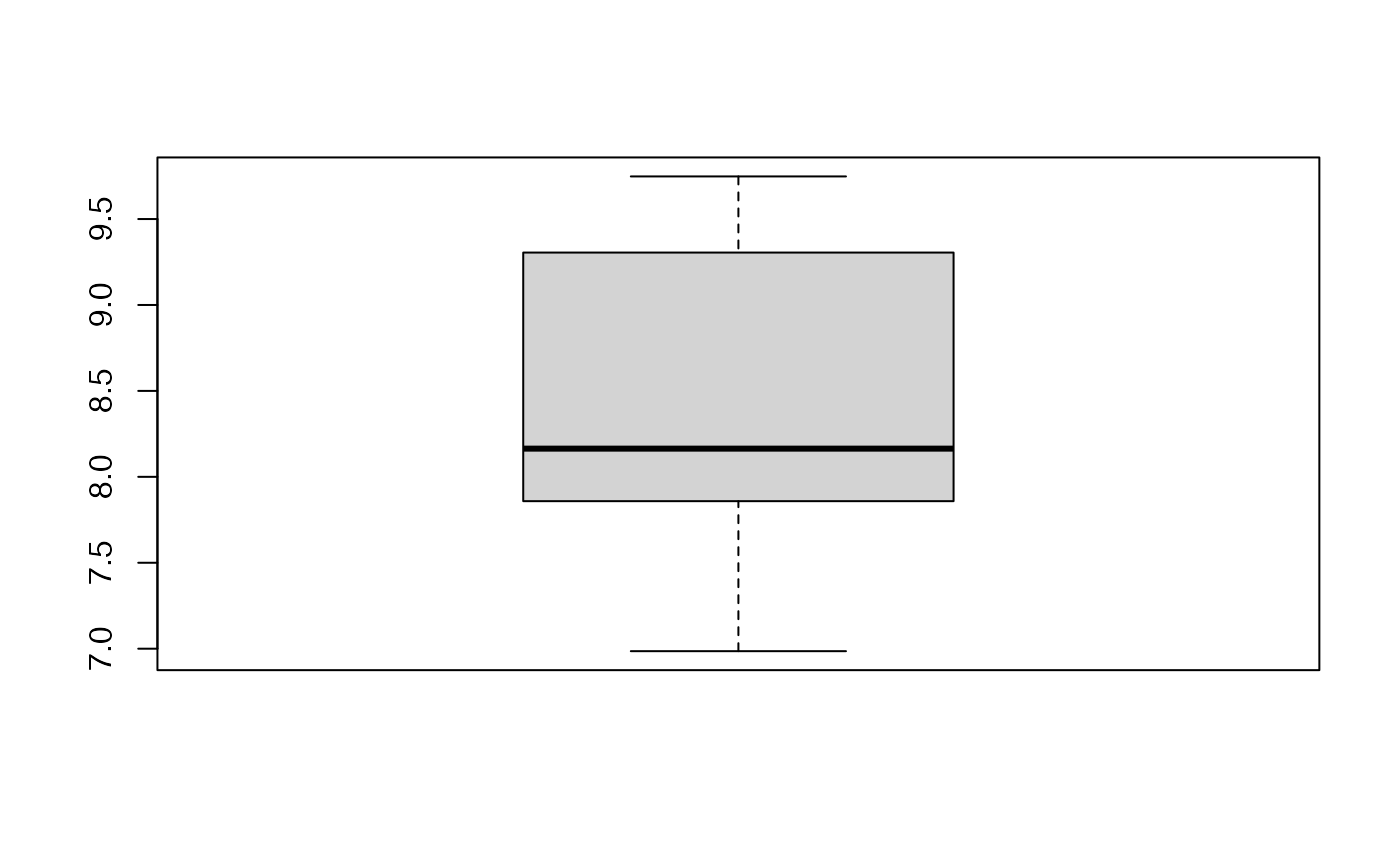 kfolds2Chisqind(bbb)
#> [[1]]
#> [[1]][[1]]
#> [1] NA NA NA NA NA NA NA NA NA NA
#>
#> [[1]][[2]]
#> [1] NA NA NA NA NA NA NA NA NA NA
#>
#> [[1]][[3]]
#> [1] NA NA NA NA NA NA NA NA NA NA
#>
#> [[1]][[4]]
#> [1] NA NA NA NA NA NA NA NA NA NA
#>
#> [[1]][[5]]
#> [1] NA NA NA NA NA NA NA NA NA NA
#>
#> [[1]][[6]]
#> [1] NA NA NA NA NA NA NA NA NA NA
#>
#> [[1]][[7]]
#> [1] NA NA NA NA NA NA NA NA NA NA
#>
#> [[1]][[8]]
#> [1] NA NA NA NA NA NA NA NA NA NA
#>
#> [[1]][[9]]
#> [1] NA NA NA NA NA NA NA NA NA NA
#>
#> [[1]][[10]]
#> [1] NA NA NA NA NA NA NA NA NA NA
#>
#>
kfolds2Chisq(bbb)
#> [[1]]
#> [1] NA NA NA NA NA NA NA NA NA NA
#>
summary(bbb)
#> ____************************************************____
#>
#> Family: gaussian
#> Link function: identity
#>
#> ____Component____ 1 ____
#> ____Component____ 2 ____
#> ____Component____ 3 ____
#> ____Component____ 4 ____
#> ____Component____ 5 ____
#> ____Component____ 6 ____
#> ____Component____ 7 ____
#> ____Component____ 8 ____
#> ____Component____ 9 ____
#> ____Component____ 10 ____
#> ____Predicting X without NA neither in X or Y____
#> ****________________________________________________****
#>
#>
#> NK: 1
#> [[1]]
#> AIC BIC Q2Chisqcum_Y limQ2 Q2Chisq_Y PREChi2_Pearson_Y
#> Nb_Comp_0 82.41888 85.41190 NA NA NA NA
#> Nb_Comp_1 63.61896 68.10848 NA 0.0975 NA NA
#> Nb_Comp_2 54.15489 60.14092 NA 0.0975 NA NA
#> Nb_Comp_3 53.47303 60.95556 NA 0.0975 NA NA
#> Nb_Comp_4 54.83398 63.81302 NA 0.0975 NA NA
#> Nb_Comp_5 56.32757 66.80312 NA 0.0975 NA NA
#> Nb_Comp_6 57.45220 69.42426 NA 0.0975 NA NA
#> Nb_Comp_7 59.31417 72.78274 NA 0.0975 NA NA
#> Nb_Comp_8 61.20356 76.16863 NA 0.0975 NA NA
#> Nb_Comp_9 63.16270 79.62429 NA 0.0975 NA NA
#> Nb_Comp_10 65.15982 83.11791 NA 0.0975 NA NA
#> Chi2_Pearson_Y RSS_Y R2_Y
#> Nb_Comp_0 20.800152 20.800152 NA
#> Nb_Comp_1 11.074659 11.074659 0.4675684
#> Nb_Comp_2 7.824528 7.824528 0.6238235
#> Nb_Comp_3 7.213793 7.213793 0.6531855
#> Nb_Comp_4 7.075441 7.075441 0.6598370
#> Nb_Comp_5 6.967693 6.967693 0.6650172
#> Nb_Comp_6 6.785296 6.785296 0.6737862
#> Nb_Comp_7 6.756973 6.756973 0.6751479
#> Nb_Comp_8 6.734363 6.734363 0.6762349
#> Nb_Comp_9 6.726030 6.726030 0.6766355
#> Nb_Comp_10 6.725443 6.725443 0.6766638
#>
#> attr(,"class")
#> [1] "summary.cv.plsRglmmodel"
PLS_lm_formula(x11~.,data=pine,nt=10,typeVC="standard")$InfCrit
#> ____************************************************____
#> ____TypeVC____ standard ____
#> ____Component____ 1 ____
#> ____Component____ 2 ____
#> ____Component____ 3 ____
#> ____Component____ 4 ____
#> ____Component____ 5 ____
#> ____Component____ 6 ____
#> ____Component____ 7 ____
#> ____Component____ 8 ____
#> ____Component____ 9 ____
#> ____Component____ 10 ____
#> ____Predicting X without NA neither in X nor in Y____
#> ****________________________________________________****
#>
#> AIC Q2cum_Y LimQ2_Y Q2_Y PRESS_Y RSS_Y
#> Nb_Comp_0 82.41888 NA NA NA NA 20.800152
#> Nb_Comp_1 63.61896 0.38248575 0.0975 0.38248575 12.844390 11.074659
#> Nb_Comp_2 58.47638 0.34836456 0.0975 -0.05525570 11.686597 8.919303
#> Nb_Comp_3 56.55421 0.23688359 0.0975 -0.17107874 10.445206 7.919786
#> Nb_Comp_4 54.35053 0.06999681 0.0975 -0.21869112 9.651773 6.972542
#> Nb_Comp_5 55.99834 -0.07691053 0.0975 -0.15796434 8.073955 6.898523
#> Nb_Comp_6 57.69592 -0.19968885 0.0975 -0.11400977 7.685022 6.835594
#> Nb_Comp_7 59.37953 -0.27722139 0.0975 -0.06462721 7.277359 6.770369
#> Nb_Comp_8 61.21213 -0.30602578 0.0975 -0.02255238 6.923057 6.736112
#> Nb_Comp_9 63.18426 -0.39920228 0.0975 -0.07134354 7.216690 6.730426
#> Nb_Comp_10 65.15982 -0.43743644 0.0975 -0.02732569 6.914340 6.725443
#> R2_Y R2_residY RSS_residY PRESS_residY Q2_residY LimQ2
#> Nb_Comp_0 NA NA 32.00000 NA NA NA
#> Nb_Comp_1 0.4675684 0.4675684 17.03781 19.76046 0.38248575 0.0975
#> Nb_Comp_2 0.5711905 0.5711905 13.72190 17.97925 -0.05525570 0.0975
#> Nb_Comp_3 0.6192438 0.6192438 12.18420 16.06943 -0.17107874 0.0975
#> Nb_Comp_4 0.6647841 0.6647841 10.72691 14.84877 -0.21869112 0.0975
#> Nb_Comp_5 0.6683426 0.6683426 10.61304 12.42138 -0.15796434 0.0975
#> Nb_Comp_6 0.6713681 0.6713681 10.51622 11.82303 -0.11400977 0.0975
#> Nb_Comp_7 0.6745039 0.6745039 10.41588 11.19586 -0.06462721 0.0975
#> Nb_Comp_8 0.6761508 0.6761508 10.36317 10.65078 -0.02255238 0.0975
#> Nb_Comp_9 0.6764242 0.6764242 10.35443 11.10252 -0.07134354 0.0975
#> Nb_Comp_10 0.6766638 0.6766638 10.34676 10.63737 -0.02732569 0.0975
#> Q2cum_residY AIC.std DoF.dof sigmahat.dof AIC.dof BIC.dof
#> Nb_Comp_0 NA 96.63448 1.000000 0.8062287 0.6697018 0.6991787
#> Nb_Comp_1 0.38248575 77.83455 3.176360 0.5994089 0.4047616 0.4565153
#> Nb_Comp_2 0.34836456 72.69198 7.133559 0.5761829 0.4138120 0.5212090
#> Nb_Comp_3 0.23688359 70.76981 8.778329 0.5603634 0.4070516 0.5320535
#> Nb_Comp_4 0.06999681 68.56612 8.427874 0.5221703 0.3505594 0.4547689
#> Nb_Comp_5 -0.07691053 70.21393 9.308247 0.5285695 0.3666578 0.4845912
#> Nb_Comp_6 -0.19968885 71.91152 9.291931 0.5259794 0.3629363 0.4795121
#> Nb_Comp_7 -0.27722139 73.59512 9.756305 0.5284535 0.3702885 0.4938445
#> Nb_Comp_8 -0.30602578 75.42772 10.363948 0.5338475 0.3831339 0.5170783
#> Nb_Comp_9 -0.39920228 77.39986 10.732146 0.5378276 0.3920957 0.5328746
#> Nb_Comp_10 -0.43743644 79.37542 11.000000 0.5407500 0.3987417 0.5446065
#> GMDL.dof DoF.naive sigmahat.naive AIC.naive BIC.naive GMDL.naive
#> Nb_Comp_0 -3.605128 1 0.8062287 0.6697018 0.6991787 -3.605128
#> Nb_Comp_1 -9.875081 2 0.5977015 0.3788984 0.4112998 -11.451340
#> Nb_Comp_2 -6.985517 3 0.5452615 0.3243383 0.3647862 -12.822703
#> Nb_Comp_3 -6.260610 4 0.5225859 0.3061986 0.3557368 -12.756838
#> Nb_Comp_4 -8.152986 5 0.4990184 0.2867496 0.3432131 -12.811575
#> Nb_Comp_5 -7.111583 6 0.5054709 0.3019556 0.3714754 -11.329638
#> Nb_Comp_6 -7.233043 7 0.5127450 0.3186757 0.4021333 -9.918688
#> Nb_Comp_7 -6.742195 8 0.5203986 0.3364668 0.4347156 -8.592770
#> Nb_Comp_8 -6.038372 9 0.5297842 0.3572181 0.4717708 -7.287834
#> Nb_Comp_9 -5.600237 10 0.5409503 0.3813021 0.5140048 -6.008747
#> Nb_Comp_10 -5.288422 11 0.5529032 0.4076026 0.5600977 -4.799453
data(pineNAX21)
bbb2 <- cv.plsRglm(x11~.,data=pineNAX21,nt=10,
modele="pls-glm-family",family=gaussian(log),K=10,keepcoeffs=TRUE,keepfolds=FALSE,verbose=FALSE)
#> Warning: glm.fit: algorithm did not converge
#> Warning: glm.fit: algorithm did not converge
#> Warning: glm.fit: algorithm did not converge
#> Warning: glm.fit: algorithm did not converge
#> Warning: glm.fit: algorithm did not converge
#> Warning: glm.fit: algorithm did not converge
#> Warning: glm.fit: algorithm did not converge
#> Warning: glm.fit: algorithm did not converge
#> Warning: glm.fit: algorithm did not converge
#> Warning: glm.fit: algorithm did not converge
#> Warning: glm.fit: algorithm did not converge
#> Warning: glm.fit: algorithm did not converge
#> Warning: glm.fit: algorithm did not converge
#> Warning: glm.fit: algorithm did not converge
#> Warning: glm.fit: algorithm did not converge
#> Warning: glm.fit: algorithm did not converge
#> Warning: glm.fit: algorithm did not converge
#> Warning: glm.fit: algorithm did not converge
#> Warning: glm.fit: algorithm did not converge
#> Warning: glm.fit: algorithm did not converge
bbb2 <- cv.plsRglm(x11~.,data=pineNAX21,nt=10,
modele="pls-glm-gaussian",K=10,keepcoeffs=TRUE,keepfolds=FALSE,verbose=FALSE)
#For Jackknife computations
kfolds2coeff(bbb2)
#> [,1] [,2] [,3] [,4] [,5] [,6]
#> [1,] 9.417696 -0.003085519 -0.03292365 0.081998660 -0.8184090 0.19049980
#> [2,] 7.145708 -0.002834763 -0.02678488 0.007015912 -0.3495267 0.08573336
#> [3,] 8.817251 -0.003483655 -0.03351176 0.091086187 -0.4417299 0.11033386
#> [4,] 8.622256 -0.003640537 -0.02347172 0.066090708 -0.5491435 0.14689903
#> [5,] 7.747370 -0.003093857 -0.03153373 0.053811988 -0.6004494 0.12626423
#> [6,] 7.317040 -0.002601577 -0.03656803 0.031504671 -0.6394931 0.12915114
#> [7,] 7.219156 -0.002823633 -0.03491071 0.016672955 -0.4603733 0.11156140
#> [8,] 9.296004 -0.003476210 -0.03318613 0.095264146 -0.6903655 0.13611562
#> [9,] 7.748634 -0.003134650 -0.03015868 0.052055792 -0.5073365 0.11210967
#> [10,] 7.052572 -0.002695906 -0.03075540 0.019841606 -0.5949681 0.12257379
#> [,7] [,8] [,9] [,10] [,11]
#> [1,] -0.76515582 -1.113753776 0.042258992 -0.2870644 -0.6195097
#> [2,] 0.35323924 -0.453700941 -0.001620362 -0.9331617 -0.2876929
#> [3,] -0.94698645 -0.130691076 0.015035900 -0.6366736 -0.5886837
#> [4,] -0.49671881 -0.191433470 -0.018161853 -0.6552005 -0.5806575
#> [5,] -0.29506311 0.241657428 0.025942148 -0.7431118 -0.7081757
#> [6,] -0.04158871 -0.130602216 0.076694670 -0.9206700 -0.4439884
#> [7,] 0.17786780 -0.006821097 -0.037157408 -0.5816967 -0.2203753
#> [8,] -0.90468636 0.249695617 0.068564185 -0.7575834 -0.9584379
#> [9,] -0.27249346 0.042666152 0.026255077 -0.7869057 -0.5688790
#> [10,] -0.02787941 -0.295338724 0.051259453 -0.6910382 -0.2890005
boxplot(kfolds2coeff(bbb2)[,1])
kfolds2Chisqind(bbb)
#> [[1]]
#> [[1]][[1]]
#> [1] NA NA NA NA NA NA NA NA NA NA
#>
#> [[1]][[2]]
#> [1] NA NA NA NA NA NA NA NA NA NA
#>
#> [[1]][[3]]
#> [1] NA NA NA NA NA NA NA NA NA NA
#>
#> [[1]][[4]]
#> [1] NA NA NA NA NA NA NA NA NA NA
#>
#> [[1]][[5]]
#> [1] NA NA NA NA NA NA NA NA NA NA
#>
#> [[1]][[6]]
#> [1] NA NA NA NA NA NA NA NA NA NA
#>
#> [[1]][[7]]
#> [1] NA NA NA NA NA NA NA NA NA NA
#>
#> [[1]][[8]]
#> [1] NA NA NA NA NA NA NA NA NA NA
#>
#> [[1]][[9]]
#> [1] NA NA NA NA NA NA NA NA NA NA
#>
#> [[1]][[10]]
#> [1] NA NA NA NA NA NA NA NA NA NA
#>
#>
kfolds2Chisq(bbb)
#> [[1]]
#> [1] NA NA NA NA NA NA NA NA NA NA
#>
summary(bbb)
#> ____************************************************____
#>
#> Family: gaussian
#> Link function: identity
#>
#> ____Component____ 1 ____
#> ____Component____ 2 ____
#> ____Component____ 3 ____
#> ____Component____ 4 ____
#> ____Component____ 5 ____
#> ____Component____ 6 ____
#> ____Component____ 7 ____
#> ____Component____ 8 ____
#> ____Component____ 9 ____
#> ____Component____ 10 ____
#> ____Predicting X without NA neither in X or Y____
#> ****________________________________________________****
#>
#>
#> NK: 1
#> [[1]]
#> AIC BIC Q2Chisqcum_Y limQ2 Q2Chisq_Y PREChi2_Pearson_Y
#> Nb_Comp_0 82.41888 85.41190 NA NA NA NA
#> Nb_Comp_1 63.61896 68.10848 NA 0.0975 NA NA
#> Nb_Comp_2 54.15489 60.14092 NA 0.0975 NA NA
#> Nb_Comp_3 53.47303 60.95556 NA 0.0975 NA NA
#> Nb_Comp_4 54.83398 63.81302 NA 0.0975 NA NA
#> Nb_Comp_5 56.32757 66.80312 NA 0.0975 NA NA
#> Nb_Comp_6 57.45220 69.42426 NA 0.0975 NA NA
#> Nb_Comp_7 59.31417 72.78274 NA 0.0975 NA NA
#> Nb_Comp_8 61.20356 76.16863 NA 0.0975 NA NA
#> Nb_Comp_9 63.16270 79.62429 NA 0.0975 NA NA
#> Nb_Comp_10 65.15982 83.11791 NA 0.0975 NA NA
#> Chi2_Pearson_Y RSS_Y R2_Y
#> Nb_Comp_0 20.800152 20.800152 NA
#> Nb_Comp_1 11.074659 11.074659 0.4675684
#> Nb_Comp_2 7.824528 7.824528 0.6238235
#> Nb_Comp_3 7.213793 7.213793 0.6531855
#> Nb_Comp_4 7.075441 7.075441 0.6598370
#> Nb_Comp_5 6.967693 6.967693 0.6650172
#> Nb_Comp_6 6.785296 6.785296 0.6737862
#> Nb_Comp_7 6.756973 6.756973 0.6751479
#> Nb_Comp_8 6.734363 6.734363 0.6762349
#> Nb_Comp_9 6.726030 6.726030 0.6766355
#> Nb_Comp_10 6.725443 6.725443 0.6766638
#>
#> attr(,"class")
#> [1] "summary.cv.plsRglmmodel"
PLS_lm_formula(x11~.,data=pine,nt=10,typeVC="standard")$InfCrit
#> ____************************************************____
#> ____TypeVC____ standard ____
#> ____Component____ 1 ____
#> ____Component____ 2 ____
#> ____Component____ 3 ____
#> ____Component____ 4 ____
#> ____Component____ 5 ____
#> ____Component____ 6 ____
#> ____Component____ 7 ____
#> ____Component____ 8 ____
#> ____Component____ 9 ____
#> ____Component____ 10 ____
#> ____Predicting X without NA neither in X nor in Y____
#> ****________________________________________________****
#>
#> AIC Q2cum_Y LimQ2_Y Q2_Y PRESS_Y RSS_Y
#> Nb_Comp_0 82.41888 NA NA NA NA 20.800152
#> Nb_Comp_1 63.61896 0.38248575 0.0975 0.38248575 12.844390 11.074659
#> Nb_Comp_2 58.47638 0.34836456 0.0975 -0.05525570 11.686597 8.919303
#> Nb_Comp_3 56.55421 0.23688359 0.0975 -0.17107874 10.445206 7.919786
#> Nb_Comp_4 54.35053 0.06999681 0.0975 -0.21869112 9.651773 6.972542
#> Nb_Comp_5 55.99834 -0.07691053 0.0975 -0.15796434 8.073955 6.898523
#> Nb_Comp_6 57.69592 -0.19968885 0.0975 -0.11400977 7.685022 6.835594
#> Nb_Comp_7 59.37953 -0.27722139 0.0975 -0.06462721 7.277359 6.770369
#> Nb_Comp_8 61.21213 -0.30602578 0.0975 -0.02255238 6.923057 6.736112
#> Nb_Comp_9 63.18426 -0.39920228 0.0975 -0.07134354 7.216690 6.730426
#> Nb_Comp_10 65.15982 -0.43743644 0.0975 -0.02732569 6.914340 6.725443
#> R2_Y R2_residY RSS_residY PRESS_residY Q2_residY LimQ2
#> Nb_Comp_0 NA NA 32.00000 NA NA NA
#> Nb_Comp_1 0.4675684 0.4675684 17.03781 19.76046 0.38248575 0.0975
#> Nb_Comp_2 0.5711905 0.5711905 13.72190 17.97925 -0.05525570 0.0975
#> Nb_Comp_3 0.6192438 0.6192438 12.18420 16.06943 -0.17107874 0.0975
#> Nb_Comp_4 0.6647841 0.6647841 10.72691 14.84877 -0.21869112 0.0975
#> Nb_Comp_5 0.6683426 0.6683426 10.61304 12.42138 -0.15796434 0.0975
#> Nb_Comp_6 0.6713681 0.6713681 10.51622 11.82303 -0.11400977 0.0975
#> Nb_Comp_7 0.6745039 0.6745039 10.41588 11.19586 -0.06462721 0.0975
#> Nb_Comp_8 0.6761508 0.6761508 10.36317 10.65078 -0.02255238 0.0975
#> Nb_Comp_9 0.6764242 0.6764242 10.35443 11.10252 -0.07134354 0.0975
#> Nb_Comp_10 0.6766638 0.6766638 10.34676 10.63737 -0.02732569 0.0975
#> Q2cum_residY AIC.std DoF.dof sigmahat.dof AIC.dof BIC.dof
#> Nb_Comp_0 NA 96.63448 1.000000 0.8062287 0.6697018 0.6991787
#> Nb_Comp_1 0.38248575 77.83455 3.176360 0.5994089 0.4047616 0.4565153
#> Nb_Comp_2 0.34836456 72.69198 7.133559 0.5761829 0.4138120 0.5212090
#> Nb_Comp_3 0.23688359 70.76981 8.778329 0.5603634 0.4070516 0.5320535
#> Nb_Comp_4 0.06999681 68.56612 8.427874 0.5221703 0.3505594 0.4547689
#> Nb_Comp_5 -0.07691053 70.21393 9.308247 0.5285695 0.3666578 0.4845912
#> Nb_Comp_6 -0.19968885 71.91152 9.291931 0.5259794 0.3629363 0.4795121
#> Nb_Comp_7 -0.27722139 73.59512 9.756305 0.5284535 0.3702885 0.4938445
#> Nb_Comp_8 -0.30602578 75.42772 10.363948 0.5338475 0.3831339 0.5170783
#> Nb_Comp_9 -0.39920228 77.39986 10.732146 0.5378276 0.3920957 0.5328746
#> Nb_Comp_10 -0.43743644 79.37542 11.000000 0.5407500 0.3987417 0.5446065
#> GMDL.dof DoF.naive sigmahat.naive AIC.naive BIC.naive GMDL.naive
#> Nb_Comp_0 -3.605128 1 0.8062287 0.6697018 0.6991787 -3.605128
#> Nb_Comp_1 -9.875081 2 0.5977015 0.3788984 0.4112998 -11.451340
#> Nb_Comp_2 -6.985517 3 0.5452615 0.3243383 0.3647862 -12.822703
#> Nb_Comp_3 -6.260610 4 0.5225859 0.3061986 0.3557368 -12.756838
#> Nb_Comp_4 -8.152986 5 0.4990184 0.2867496 0.3432131 -12.811575
#> Nb_Comp_5 -7.111583 6 0.5054709 0.3019556 0.3714754 -11.329638
#> Nb_Comp_6 -7.233043 7 0.5127450 0.3186757 0.4021333 -9.918688
#> Nb_Comp_7 -6.742195 8 0.5203986 0.3364668 0.4347156 -8.592770
#> Nb_Comp_8 -6.038372 9 0.5297842 0.3572181 0.4717708 -7.287834
#> Nb_Comp_9 -5.600237 10 0.5409503 0.3813021 0.5140048 -6.008747
#> Nb_Comp_10 -5.288422 11 0.5529032 0.4076026 0.5600977 -4.799453
data(pineNAX21)
bbb2 <- cv.plsRglm(x11~.,data=pineNAX21,nt=10,
modele="pls-glm-family",family=gaussian(log),K=10,keepcoeffs=TRUE,keepfolds=FALSE,verbose=FALSE)
#> Warning: glm.fit: algorithm did not converge
#> Warning: glm.fit: algorithm did not converge
#> Warning: glm.fit: algorithm did not converge
#> Warning: glm.fit: algorithm did not converge
#> Warning: glm.fit: algorithm did not converge
#> Warning: glm.fit: algorithm did not converge
#> Warning: glm.fit: algorithm did not converge
#> Warning: glm.fit: algorithm did not converge
#> Warning: glm.fit: algorithm did not converge
#> Warning: glm.fit: algorithm did not converge
#> Warning: glm.fit: algorithm did not converge
#> Warning: glm.fit: algorithm did not converge
#> Warning: glm.fit: algorithm did not converge
#> Warning: glm.fit: algorithm did not converge
#> Warning: glm.fit: algorithm did not converge
#> Warning: glm.fit: algorithm did not converge
#> Warning: glm.fit: algorithm did not converge
#> Warning: glm.fit: algorithm did not converge
#> Warning: glm.fit: algorithm did not converge
#> Warning: glm.fit: algorithm did not converge
bbb2 <- cv.plsRglm(x11~.,data=pineNAX21,nt=10,
modele="pls-glm-gaussian",K=10,keepcoeffs=TRUE,keepfolds=FALSE,verbose=FALSE)
#For Jackknife computations
kfolds2coeff(bbb2)
#> [,1] [,2] [,3] [,4] [,5] [,6]
#> [1,] 9.417696 -0.003085519 -0.03292365 0.081998660 -0.8184090 0.19049980
#> [2,] 7.145708 -0.002834763 -0.02678488 0.007015912 -0.3495267 0.08573336
#> [3,] 8.817251 -0.003483655 -0.03351176 0.091086187 -0.4417299 0.11033386
#> [4,] 8.622256 -0.003640537 -0.02347172 0.066090708 -0.5491435 0.14689903
#> [5,] 7.747370 -0.003093857 -0.03153373 0.053811988 -0.6004494 0.12626423
#> [6,] 7.317040 -0.002601577 -0.03656803 0.031504671 -0.6394931 0.12915114
#> [7,] 7.219156 -0.002823633 -0.03491071 0.016672955 -0.4603733 0.11156140
#> [8,] 9.296004 -0.003476210 -0.03318613 0.095264146 -0.6903655 0.13611562
#> [9,] 7.748634 -0.003134650 -0.03015868 0.052055792 -0.5073365 0.11210967
#> [10,] 7.052572 -0.002695906 -0.03075540 0.019841606 -0.5949681 0.12257379
#> [,7] [,8] [,9] [,10] [,11]
#> [1,] -0.76515582 -1.113753776 0.042258992 -0.2870644 -0.6195097
#> [2,] 0.35323924 -0.453700941 -0.001620362 -0.9331617 -0.2876929
#> [3,] -0.94698645 -0.130691076 0.015035900 -0.6366736 -0.5886837
#> [4,] -0.49671881 -0.191433470 -0.018161853 -0.6552005 -0.5806575
#> [5,] -0.29506311 0.241657428 0.025942148 -0.7431118 -0.7081757
#> [6,] -0.04158871 -0.130602216 0.076694670 -0.9206700 -0.4439884
#> [7,] 0.17786780 -0.006821097 -0.037157408 -0.5816967 -0.2203753
#> [8,] -0.90468636 0.249695617 0.068564185 -0.7575834 -0.9584379
#> [9,] -0.27249346 0.042666152 0.026255077 -0.7869057 -0.5688790
#> [10,] -0.02787941 -0.295338724 0.051259453 -0.6910382 -0.2890005
boxplot(kfolds2coeff(bbb2)[,1])
 kfolds2Chisqind(bbb2)
#> [[1]]
#> [[1]][[1]]
#> [1] NA NA NA NA NA NA NA NA NA
#>
#> [[1]][[2]]
#> [1] NA NA NA NA NA NA NA NA NA
#>
#> [[1]][[3]]
#> [1] NA NA NA NA NA NA NA NA NA
#>
#> [[1]][[4]]
#> [1] NA NA NA NA NA NA NA NA NA
#>
#> [[1]][[5]]
#> [1] NA NA NA NA NA NA NA NA NA
#>
#> [[1]][[6]]
#> [1] NA NA NA NA NA NA NA NA NA
#>
#> [[1]][[7]]
#> [1] NA NA NA NA NA NA NA NA NA
#>
#> [[1]][[8]]
#> [1] NA NA NA NA NA NA NA NA NA
#>
#> [[1]][[9]]
#> [1] NA NA NA NA NA NA NA NA NA
#>
#> [[1]][[10]]
#> [1] NA NA NA NA NA NA NA NA NA
#>
#>
kfolds2Chisq(bbb2)
#> [[1]]
#> [1] NA NA NA NA NA NA NA NA NA
#>
summary(bbb2)
#> ____************************************************____
#> Only naive DoF can be used with missing data
#>
#> Family: gaussian
#> Link function: identity
#>
#> ____There are some NAs in X but not in Y____
#> ____Component____ 1 ____
#> ____Component____ 2 ____
#> ____Component____ 3 ____
#> ____Component____ 4 ____
#> ____Component____ 5 ____
#> ____Component____ 6 ____
#> ____Component____ 7 ____
#> ____Component____ 8 ____
#> ____Component____ 9 ____
#> ____Predicting X with NA in X and not in Y____
#> ****________________________________________________****
#>
#>
#> NK: 1
#> [[1]]
#> AIC BIC Q2Chisqcum_Y limQ2 Q2Chisq_Y PREChi2_Pearson_Y
#> Nb_Comp_0 82.41888 85.41190 NA NA NA NA
#> Nb_Comp_1 63.90814 68.39766 NA 0.0975 NA NA
#> Nb_Comp_2 54.06295 60.04898 NA 0.0975 NA NA
#> Nb_Comp_3 53.77276 61.25530 NA 0.0975 NA NA
#> Nb_Comp_4 55.18223 64.16127 NA 0.0975 NA NA
#> Nb_Comp_5 56.53963 67.01518 NA 0.0975 NA NA
#> Nb_Comp_6 57.73540 69.70746 NA 0.0975 NA NA
#> Nb_Comp_7 59.46634 72.93491 NA 0.0975 NA NA
#> Nb_Comp_8 60.79943 75.76451 NA 0.0975 NA NA
#> Nb_Comp_9 62.14147 78.60305 NA 0.0975 NA NA
#> Chi2_Pearson_Y RSS_Y R2_Y
#> Nb_Comp_0 20.800152 20.800152 NA
#> Nb_Comp_1 11.172133 11.172133 0.4628821
#> Nb_Comp_2 7.802760 7.802760 0.6248700
#> Nb_Comp_3 7.279614 7.279614 0.6500211
#> Nb_Comp_4 7.150504 7.150504 0.6562283
#> Nb_Comp_5 7.012612 7.012612 0.6628577
#> Nb_Comp_6 6.843775 6.843775 0.6709747
#> Nb_Comp_7 6.788203 6.788203 0.6736465
#> Nb_Comp_8 6.652395 6.652395 0.6801757
#> Nb_Comp_9 6.521071 6.521071 0.6864893
#>
#> attr(,"class")
#> [1] "summary.cv.plsRglmmodel"
PLS_lm_formula(x11~.,data=pineNAX21,nt=10,typeVC="standard")$InfCrit
#> ____************************************************____
#> Only naive DoF can be used with missing data
#> ____There are some NAs in X but not in Y____
#> ____TypeVC____ standard ____
#> ____TypeVC____ standard ____unknown____
#> ____Component____ 1 ____
#> ____Component____ 2 ____
#> ____Component____ 3 ____
#> ____Component____ 4 ____
#> ____Component____ 5 ____
#> ____Component____ 6 ____
#> ____Component____ 7 ____
#> ____Component____ 8 ____
#> ____Component____ 9 ____
#> Warning : reciprocal condition number of t(cbind(res$pp,temppp)[XXNA[1,],,drop=FALSE])%*%cbind(res$pp,temppp)[XXNA[1,],,drop=FALSE] < 10^{-12}
#> Warning only 9 components could thus be extracted
#> ____Predicting X with NA in X and not in Y____
#> ****________________________________________________****
#>
#> AIC Q2cum_Y LimQ2_Y Q2_Y PRESS_Y RSS_Y
#> Nb_Comp_0 82.41888 NA NA NA NA 20.800152
#> Nb_Comp_1 63.69250 0.35639805 0.0975 0.35639805 13.387018 11.099368
#> Nb_Comp_2 58.35228 0.28395028 0.0975 -0.11256611 12.348781 8.885823
#> Nb_Comp_3 56.36553 0.07664889 0.0975 -0.28950699 11.458331 7.874634
#> Nb_Comp_4 54.02416 -0.70355579 0.0975 -0.84497074 14.528469 6.903925
#> Nb_Comp_5 55.80450 -0.94905654 0.0975 -0.14411078 7.898855 6.858120
#> Nb_Comp_6 57.45753 -1.27568315 0.0975 -0.16758190 8.007417 6.786392
#> Nb_Comp_7 58.73951 -1.63309014 0.0975 -0.15705481 7.852227 6.640327
#> Nb_Comp_8 60.61227 -1.67907859 0.0975 -0.01746558 6.756304 6.614773
#> Nb_Comp_9 62.25948 -2.15165796 0.0975 -0.17639623 7.781594 6.544432
#> R2_Y R2_residY RSS_residY PRESS_residY Q2_residY LimQ2
#> Nb_Comp_0 NA NA 32.00000 NA NA NA
#> Nb_Comp_1 0.4663804 0.4663804 17.07583 20.59526 0.35639805 0.0975
#> Nb_Comp_2 0.5728001 0.5728001 13.67040 18.99799 -0.11256611 0.0975
#> Nb_Comp_3 0.6214146 0.6214146 12.11473 17.62807 -0.28950699 0.0975
#> Nb_Comp_4 0.6680830 0.6680830 10.62135 22.35133 -0.84497074 0.0975
#> Nb_Comp_5 0.6702851 0.6702851 10.55088 12.15200 -0.14411078 0.0975
#> Nb_Comp_6 0.6737336 0.6737336 10.44053 12.31901 -0.16758190 0.0975
#> Nb_Comp_7 0.6807558 0.6807558 10.21581 12.08026 -0.15705481 0.0975
#> Nb_Comp_8 0.6819844 0.6819844 10.17650 10.39424 -0.01746558 0.0975
#> Nb_Comp_9 0.6853661 0.6853661 10.06828 11.97160 -0.17639623 0.0975
#> Q2cum_residY AIC.std DoF.dof sigmahat.dof AIC.dof BIC.dof GMDL.dof
#> Nb_Comp_0 NA 96.63448 NA NA NA NA NA
#> Nb_Comp_1 0.35639805 77.90810 NA NA NA NA NA
#> Nb_Comp_2 0.28395028 72.56787 NA NA NA NA NA
#> Nb_Comp_3 0.07664889 70.58113 NA NA NA NA NA
#> Nb_Comp_4 -0.70355579 68.23976 NA NA NA NA NA
#> Nb_Comp_5 -0.94905654 70.02009 NA NA NA NA NA
#> Nb_Comp_6 -1.27568315 71.67313 NA NA NA NA NA
#> Nb_Comp_7 -1.63309014 72.95511 NA NA NA NA NA
#> Nb_Comp_8 -1.67907859 74.82787 NA NA NA NA NA
#> Nb_Comp_9 -2.15165796 76.47507 NA NA NA NA NA
#> DoF.naive sigmahat.naive AIC.naive BIC.naive GMDL.naive
#> Nb_Comp_0 1 0.8062287 0.6697018 0.6991787 -3.605128
#> Nb_Comp_1 2 0.5983679 0.3797438 0.4122175 -11.413749
#> Nb_Comp_2 3 0.5442372 0.3231208 0.3634169 -12.847656
#> Nb_Comp_3 4 0.5210941 0.3044529 0.3537087 -12.776843
#> Nb_Comp_4 5 0.4965569 0.2839276 0.3398355 -12.891035
#> Nb_Comp_5 6 0.5039885 0.3001871 0.3692997 -11.349498
#> Nb_Comp_6 7 0.5108963 0.3163819 0.3992388 -9.922119
#> Nb_Comp_7 8 0.5153766 0.3300041 0.4263658 -8.696873
#> Nb_Comp_8 9 0.5249910 0.3507834 0.4632727 -7.337679
#> Nb_Comp_9 10 0.5334234 0.3707649 0.4998004 -6.033403
rm(list=c("bbb","bbb2"))
data(aze_compl)
bbb <- cv.plsRglm(y~.,data=aze_compl,nt=10,K=10,modele="pls",
keepcoeffs=TRUE,verbose=FALSE)
#For Jackknife computations
kfolds2coeff(bbb)
#> [,1] [,2] [,3] [,4] [,5] [,6]
#> [1,] 0.2904228 -0.16546999 0.4613569 -0.2286029 0.3856101 0.19997604
#> [2,] 0.2788494 -0.15379671 0.2872360 -0.1616180 0.2799155 0.06554366
#> [3,] 0.2611695 -0.10970491 0.4432985 -0.1519190 0.2286516 0.16025696
#> [4,] 0.3107607 -0.09353284 0.4504198 -0.1732064 0.1558267 0.14893733
#> [5,] 0.2353885 -0.20528895 0.4614184 -0.2310755 0.3168370 0.06767269
#> [6,] 0.3838840 -0.14015351 0.4260461 -0.2183473 0.2572394 0.12343355
#> [7,] 0.4397244 -0.05753894 0.4190984 -0.1646686 0.2418824 0.08820954
#> [8,] 0.3215070 -0.15750170 0.4834184 -0.1708883 0.3484636 0.07815465
#> [9,] 0.4178985 -0.16920876 0.4723971 -0.1464944 0.1380466 0.09771230
#> [10,] 0.1603134 -0.10438813 0.5847150 -0.2461680 0.3367957 0.05361732
#> [,7] [,8] [,9] [,10] [,11] [,12]
#> [1,] -0.03147007 0.005447243 -0.25466893 0.075540157 -0.12212338 0.07503150
#> [2,] -0.04483009 0.006006823 -0.12822608 0.059277262 -0.05628416 0.01172033
#> [3,] -0.08010147 -0.004494762 -0.17458325 0.079604238 -0.03021918 -0.01326882
#> [4,] -0.07870415 0.046118297 -0.16437668 0.047937140 -0.11303248 0.05961749
#> [5,] -0.02190554 -0.035631497 -0.25287862 0.032991764 -0.12731337 0.07825341
#> [6,] -0.12150132 0.041957218 -0.27680064 -0.007849660 -0.02937310 0.09737774
#> [7,] -0.09555267 -0.004121272 -0.16888557 0.008354877 -0.10718182 0.07161800
#> [8,] 0.03342254 -0.076191370 -0.35907808 0.045943810 -0.13552329 0.08341805
#> [9,] -0.06646697 0.037302167 -0.04875343 0.006454279 -0.15806923 0.09880511
#> [10,] 0.02576205 0.057609599 -0.30717154 0.111079203 -0.11998307 0.06447860
#> [,13] [,14] [,15] [,16] [,17] [,18]
#> [1,] -0.23605039 0.09132327 0.11871387 0.05238841 0.079533632 0.2310862
#> [2,] -0.08778194 0.20025677 0.14271415 0.15825821 -0.005158815 0.1463330
#> [3,] -0.13167005 0.18791410 0.13124435 0.01007703 -0.051049524 0.2258172
#> [4,] -0.03986917 0.01164343 0.13930641 0.07874179 0.024434649 0.2053491
#> [5,] -0.08399076 0.06113521 0.12303185 0.01037210 0.025948557 0.2763917
#> [6,] -0.07048540 0.07374076 0.09789945 0.02290605 -0.025232369 0.3149448
#> [7,] -0.11999560 0.18408022 0.04962935 -0.01007692 -0.031605435 0.1593562
#> [8,] -0.16316496 0.12610938 0.04204067 0.19241795 0.057004170 0.2224195
#> [9,] -0.12803369 0.03888839 0.14377609 0.06005691 -0.027012090 0.2602918
#> [10,] -0.22418988 0.07889964 0.11437179 0.05428228 0.060792746 0.3352487
#> [,19] [,20] [,21] [,22] [,23] [,24]
#> [1,] 0.052229631 0.007385233 -0.25282651 0.056446650 0.33429850 -0.15217124
#> [2,] 0.038417870 0.107278283 -0.07953724 0.075446065 0.13550787 -0.16390057
#> [3,] 0.006927076 0.080982967 -0.10468827 0.108960415 0.18333130 -0.13508928
#> [4,] -0.022328933 0.182848961 -0.17171106 0.047373613 0.06461360 -0.11134306
#> [5,] 0.012402191 0.088233652 -0.07156676 0.136283685 0.17319692 -0.13247308
#> [6,] -0.025334581 0.122883152 -0.05858277 0.008872599 0.26877774 -0.13744291
#> [7,] 0.036579422 -0.035798152 -0.12907028 0.028579269 0.24776651 -0.20559335
#> [8,] -0.089062486 0.088824430 -0.15330373 0.025641891 0.24578349 -0.17179775
#> [9,] 0.053065315 0.052679782 -0.18413276 0.121779310 0.01200132 -0.02829972
#> [10,] 0.068251735 0.063652085 -0.09165695 0.076084106 0.22637119 -0.19472896
#> [,25] [,26] [,27] [,28] [,29] [,30]
#> [1,] -0.1964368 -0.2665771 0.1585707 0.1804507 -0.03106563 0.069155087
#> [2,] -0.1684274 -0.2475508 0.1589951 0.1262438 -0.10324404 -0.001352712
#> [3,] -0.1957547 -0.3164055 0.1924212 0.2549146 -0.09565424 0.034795798
#> [4,] -0.2086419 -0.1905443 0.2017151 0.1801214 -0.17652333 0.082746808
#> [5,] -0.1229588 -0.2931490 0.2342065 0.1693008 -0.13782128 -0.049492555
#> [6,] -0.1806949 -0.3787962 0.1944198 0.1825709 -0.10505455 0.039556420
#> [7,] -0.2023592 -0.2792575 0.1746820 0.2441362 -0.11303775 -0.007783524
#> [8,] -0.1649146 -0.2956775 0.1993148 0.2920899 -0.06420454 -0.010086608
#> [9,] -0.1756940 -0.3132950 0.1772571 0.2278046 -0.10498110 -0.043764396
#> [10,] -0.2225357 -0.3225024 0.1896744 0.1260020 -0.06321541 0.057762191
#> [,31] [,32] [,33] [,34]
#> [1,] 0.04102614 -0.07503820 -0.3786917 -0.028915111
#> [2,] 0.23692286 -0.09989328 -0.3971052 -0.053458363
#> [3,] 0.06245648 -0.03138443 -0.4016336 -0.037755788
#> [4,] 0.10169762 -0.06906329 -0.3787767 -0.032138377
#> [5,] 0.12463061 -0.03563325 -0.2891516 -0.009933863
#> [6,] 0.10843944 -0.05708189 -0.3841296 -0.032853634
#> [7,] 0.17627414 -0.07719379 -0.4426674 0.093447741
#> [8,] 0.06843106 -0.09879500 -0.2923301 0.013059072
#> [9,] 0.22575481 0.07828888 -0.5832959 -0.039093844
#> [10,] 0.11795164 -0.02646349 -0.4134898 -0.029182528
bbb2 <- cv.plsRglm(y~.,data=aze_compl,nt=3,K=10,
modele="pls-glm-family",family=binomial(probit),keepcoeffs=TRUE,verbose=FALSE)
bbb2 <- cv.plsRglm(y~.,data=aze_compl,nt=3,K=10,
modele="pls-glm-logistic",keepcoeffs=TRUE,verbose=FALSE)
summary(bbb,MClassed=TRUE)
#> ____************************************************____
#>
#> Model: pls
#>
#> ____Component____ 1 ____
#> ____Component____ 2 ____
#> ____Component____ 3 ____
#> ____Component____ 4 ____
#> ____Component____ 5 ____
#> ____Component____ 6 ____
#> ____Component____ 7 ____
#> ____Component____ 8 ____
#> ____Component____ 9 ____
#> ____Component____ 10 ____
#> ____Predicting X without NA neither in X or Y____
#> ****________________________________________________****
#>
#>
#> NK: 1
#> [[1]]
#> AIC MissClassed CV_MissClassed Q2cum_Y LimQ2_Y
#> Nb_Comp_0 154.6179 49 NA NA NA
#> Nb_Comp_1 126.4083 27 44 -0.07967991 0.0975
#> Nb_Comp_2 119.3375 25 45 -0.61560068 0.0975
#> Nb_Comp_3 114.2313 27 44 -1.79789662 0.0975
#> Nb_Comp_4 112.3463 23 44 -4.49018690 0.0975
#> Nb_Comp_5 113.2362 22 42 -10.27579259 0.0975
#> Nb_Comp_6 114.7620 21 42 -22.63990722 0.0975
#> Nb_Comp_7 116.5264 20 43 -49.21935486 0.0975
#> Nb_Comp_8 118.4601 20 43 -107.06034605 0.0975
#> Nb_Comp_9 120.4452 19 43 -232.31457561 0.0975
#> Nb_Comp_10 122.4395 19 43 -502.49592428 0.0975
#> Q2_Y PRESS_Y RSS_Y R2_Y AIC.std DoF.dof
#> Nb_Comp_0 NA NA 25.91346 NA 298.1344 1.00000
#> Nb_Comp_1 -0.07967991 27.97824 19.38086 0.2520929 269.9248 22.55372
#> Nb_Comp_2 -0.49637005 29.00094 17.76209 0.3145613 262.8540 27.31542
#> Nb_Comp_3 -0.73179960 30.76038 16.58896 0.3598323 257.7478 30.52370
#> Nb_Comp_4 -0.96225510 32.55177 15.98071 0.3833049 255.8628 34.00000
#> Nb_Comp_5 -1.05380851 32.82131 15.81104 0.3898523 256.7527 34.00000
#> Nb_Comp_6 -1.09651845 33.14814 15.73910 0.3926285 258.2785 34.00000
#> Nb_Comp_7 -1.12434653 33.43530 15.70350 0.3940024 260.0429 33.71066
#> Nb_Comp_8 -1.15176691 33.79026 15.69348 0.3943888 261.9766 34.00000
#> Nb_Comp_9 -1.15911372 33.88401 15.69123 0.3944758 263.9617 33.87284
#> Nb_Comp_10 -1.15801316 33.86188 15.69037 0.3945088 265.9560 34.00000
#> sigmahat.dof AIC.dof BIC.dof GMDL.dof DoF.naive sigmahat.naive
#> Nb_Comp_0 0.5015845 0.2540061 0.2604032 -67.17645 1 0.5015845
#> Nb_Comp_1 0.4848429 0.2883114 0.4231184 -53.56607 2 0.4358996
#> Nb_Comp_2 0.4781670 0.2908950 0.4496983 -52.42272 3 0.4193593
#> Nb_Comp_3 0.4719550 0.2902572 0.4631316 -51.93343 4 0.4072955
#> Nb_Comp_4 0.4744263 0.3008285 0.4954133 -50.37079 5 0.4017727
#> Nb_Comp_5 0.4719012 0.2976347 0.4901536 -50.65724 6 0.4016679
#> Nb_Comp_6 0.4708264 0.2962804 0.4879234 -50.78005 7 0.4028135
#> Nb_Comp_7 0.4693382 0.2937976 0.4826103 -51.05525 8 0.4044479
#> Nb_Comp_8 0.4701436 0.2954217 0.4865092 -50.85833 9 0.4064413
#> Nb_Comp_9 0.4696894 0.2945815 0.4845867 -50.95616 10 0.4085682
#> Nb_Comp_10 0.4700970 0.2953632 0.4864128 -50.86368 11 0.4107477
#> AIC.naive BIC.naive GMDL.naive
#> Nb_Comp_0 0.2540061 0.2604032 -67.17645
#> Nb_Comp_1 0.1936625 0.2033251 -79.67755
#> Nb_Comp_2 0.1809352 0.1943501 -81.93501
#> Nb_Comp_3 0.1722700 0.1891422 -83.31503
#> Nb_Comp_4 0.1691819 0.1897041 -83.23369
#> Nb_Comp_5 0.1706451 0.1952588 -81.93513
#> Nb_Comp_6 0.1731800 0.2020601 -80.42345
#> Nb_Comp_7 0.1761610 0.2094352 -78.87607
#> Nb_Comp_8 0.1794902 0.2172936 -77.31942
#> Nb_Comp_9 0.1829787 0.2254232 -75.80069
#> Nb_Comp_10 0.1865584 0.2337468 -74.33325
#>
#> attr(,"class")
#> [1] "summary.cv.plsRmodel"
summary(bbb2,MClassed=TRUE)
#> ____************************************************____
#>
#> Family: binomial
#> Link function: logit
#>
#> ____Component____ 1 ____
#> ____Component____ 2 ____
#> ____Component____ 3 ____
#> ____Predicting X without NA neither in X or Y____
#> ****________________________________________________****
#>
#>
#> NK: 1
#> [[1]]
#> AIC BIC MissClassed CV_MissClassed Q2Chisqcum_Y limQ2
#> Nb_Comp_0 145.8283 148.4727 49 NA NA NA
#> Nb_Comp_1 118.1398 123.4285 28 NA NA 0.0975
#> Nb_Comp_2 109.9553 117.8885 26 NA NA 0.0975
#> Nb_Comp_3 105.1591 115.7366 22 NA NA 0.0975
#> Q2Chisq_Y PREChi2_Pearson_Y Chi2_Pearson_Y RSS_Y R2_Y
#> Nb_Comp_0 NA NA 104.00000 25.91346 NA
#> Nb_Comp_1 NA NA 100.53823 19.32272 0.2543365
#> Nb_Comp_2 NA NA 99.17955 17.33735 0.3309519
#> Nb_Comp_3 NA NA 123.37836 15.58198 0.3986915
#>
#> attr(,"class")
#> [1] "summary.cv.plsRglmmodel"
kfolds2coeff(bbb2)
#> [,1] [,2] [,3] [,4] [,5] [,6]
#> [1,] -0.5856366 -0.70593213 1.852552 -0.3050775 0.9084177 -0.18877819
#> [2,] -0.8149337 -0.73838107 2.763618 -0.4614720 0.9635515 -0.04805976
#> [3,] -1.2104711 -0.32395091 2.662943 -0.6279237 0.6450661 -0.05595700
#> [4,] -2.1711113 -0.50606432 1.759972 -0.4426020 1.3427648 0.64588373
#> [5,] -1.9935056 0.06530008 1.770743 -0.5783879 1.3377936 -0.17958544
#> [6,] -1.4859983 -0.53089451 2.462009 -0.5974124 0.9383782 0.23660079
#> [7,] -0.3864483 -0.60078416 2.859719 -0.5107874 1.6598961 0.41849554
#> [8,] -1.6510734 0.27315603 3.038843 0.3358956 0.7353031 -0.34258677
#> [9,] -0.1003971 -0.89129549 2.183817 -0.3697520 0.4157663 0.17963575
#> [10,] -0.6625460 -0.64377729 2.526018 -0.6559876 0.9569176 -0.10450252
#> [,7] [,8] [,9] [,10] [,11] [,12]
#> [1,] 0.008477155 0.25577898 -0.5714143 -0.1721756 -0.7181097 0.29542011
#> [2,] -0.986938549 0.03781580 -0.3094900 0.2855071 -0.5693793 -0.18382052
#> [3,] -0.251958563 -0.51486260 -0.6625394 0.3355462 -0.2945604 0.38942886
#> [4,] -0.510662840 0.36978247 -0.3460350 -0.3202278 -0.8925107 0.53442304
#> [5,] -0.355457619 0.28457491 -0.7914298 0.1330579 -0.9832421 -0.08610594
#> [6,] -0.845401022 0.45731976 -0.6975156 0.1994099 -0.6196171 -0.50806788
#> [7,] -0.965694039 -0.15612775 -0.9140809 -0.6073345 -0.7170569 -0.13182391
#> [8,] -0.618266882 0.68708061 -1.1213766 0.4119966 -0.6572498 -0.27936091
#> [9,] -0.732194986 0.06256693 -0.6381877 0.1896016 -0.8825244 -0.17045254
#> [10,] -0.745248026 0.39187113 -0.7105860 0.6766861 -0.4629398 -0.15548511
#> [,13] [,14] [,15] [,16] [,17] [,18]
#> [1,] -0.4677350 1.0126091 1.3258372 0.8628136 0.194131085 0.6326976
#> [2,] -0.3216674 0.4738930 1.6062460 0.1129500 0.300569466 1.4939696
#> [3,] -0.4222692 0.3927179 1.0300889 0.2752369 -0.348980574 1.4146577
#> [4,] -0.6229572 0.9921400 1.4742803 0.3985643 -0.252523176 1.4527357
#> [5,] -0.4068965 0.8343620 1.6595472 0.5022135 0.110644396 0.5872420
#> [6,] -0.5202251 1.1988388 1.1544251 0.5638662 -0.080060451 0.9634235
#> [7,] -0.4290171 1.1734399 0.8459654 0.8235340 -0.124221608 0.7714531
#> [8,] -0.5769116 0.4822520 0.9691335 0.6861565 -0.047622093 1.2112867
#> [9,] -0.1023990 0.6408009 0.9996327 0.1723059 0.072142725 1.1117595
#> [10,] -0.5754584 0.6461705 0.7156629 0.6338462 0.005688769 0.9835615
#> [,19] [,20] [,21] [,22] [,23] [,24]
#> [1,] 0.04211886 0.4712776 -0.8024290 0.33306839 0.9916961 -0.4896372
#> [2,] -0.31380722 1.0799777 -0.9825220 0.40162252 0.4462640 -0.4953247
#> [3,] 0.23966705 0.7437650 -0.5270733 0.59611897 0.4822368 -0.9027950
#> [4,] 0.27264659 0.2713775 -0.9791310 0.04606772 0.5686849 -0.6341368
#> [5,] -0.17400214 0.5198480 -0.8645098 0.47231855 0.4960366 -0.5216491
#> [6,] -0.05327875 0.8808986 -0.6839469 0.04770620 1.0180354 -1.0647194
#> [7,] 0.34305492 0.7716648 -0.6110081 -0.10219774 0.7983989 -0.8266582
#> [8,] 0.44811485 1.1579532 -0.8321312 -0.25480175 0.7151986 -1.0043173
#> [9,] 0.02639448 0.6706990 -1.2267333 0.49189615 1.5613934 -0.4508710
#> [10,] 0.51225877 0.4497280 -0.8426358 0.33018067 0.4243222 -0.5258497
#> [,25] [,26] [,27] [,28] [,29] [,30]
#> [1,] -1.0528126 -1.093123 0.2301459 1.1119871 -1.2893685 -0.252093424
#> [2,] -0.7105976 -1.244015 0.7649467 0.4726965 -0.6243811 -0.617331695
#> [3,] -0.7793126 -1.427220 0.5230731 0.7290150 -1.3367052 -0.333563870
#> [4,] -0.8968540 -1.552835 0.4248156 1.0669958 -1.2727016 -0.338020891
#> [5,] -1.0773448 -1.315935 0.5379118 0.6151999 -0.6221073 -0.497233136
#> [6,] -0.9794836 -1.410567 0.7320261 1.1101333 -0.9543077 0.031837790
#> [7,] -1.5409095 -1.361478 1.1317922 0.9686751 -1.0120843 0.001022957
#> [8,] -1.6981563 -1.321080 0.6577176 0.6252492 -1.0105108 -0.287975245
#> [9,] -1.9329688 -1.384525 0.7801307 1.3864025 -1.4512861 0.062855637
#> [10,] -1.3367175 -1.550137 0.3331949 0.7286957 -0.9973156 0.002383937
#> [,31] [,32] [,33] [,34]
#> [1,] 0.4374923 0.39035300 -2.005615 -0.56751270
#> [2,] 0.8935647 0.92683013 -3.433172 0.05492884
#> [3,] 0.9212239 0.41337778 -1.953009 0.02387227
#> [4,] 1.9460768 0.47684686 -2.389454 -0.03604205
#> [5,] 1.5763427 0.57492711 -1.512309 -0.09687232
#> [6,] 1.0673302 0.31128852 -2.564469 0.17118097
#> [7,] 0.8383126 -0.16979131 -2.321932 -0.14154021
#> [8,] 1.1259856 0.80665697 -2.443683 -0.24572429
#> [9,] 1.0663707 0.06049022 -2.333540 0.12834523
#> [10,] 1.3432225 0.28651553 -2.245218 -0.05168191
kfolds2Chisqind(bbb2)
#> [[1]]
#> [[1]][[1]]
#> [1] NA NA NA
#>
#> [[1]][[2]]
#> [1] NA NA NA
#>
#> [[1]][[3]]
#> [1] NA NA NA
#>
#> [[1]][[4]]
#> [1] NA NA NA
#>
#> [[1]][[5]]
#> [1] NA NA NA
#>
#> [[1]][[6]]
#> [1] NA NA NA
#>
#> [[1]][[7]]
#> [1] NA NA NA
#>
#> [[1]][[8]]
#> [1] NA NA NA
#>
#> [[1]][[9]]
#> [1] NA NA NA
#>
#> [[1]][[10]]
#> [1] NA NA NA
#>
#>
kfolds2Chisq(bbb2)
#> [[1]]
#> [1] NA NA NA
#>
summary(bbb2)
#> ____************************************************____
#>
#> Family: binomial
#> Link function: logit
#>
#> ____Component____ 1 ____
#> ____Component____ 2 ____
#> ____Component____ 3 ____
#> ____Predicting X without NA neither in X or Y____
#> ****________________________________________________****
#>
#>
#> NK: 1
#> [[1]]
#> AIC BIC Q2Chisqcum_Y limQ2 Q2Chisq_Y PREChi2_Pearson_Y
#> Nb_Comp_0 145.8283 148.4727 NA NA NA NA
#> Nb_Comp_1 118.1398 123.4285 NA 0.0975 NA NA
#> Nb_Comp_2 109.9553 117.8885 NA 0.0975 NA NA
#> Nb_Comp_3 105.1591 115.7366 NA 0.0975 NA NA
#> Chi2_Pearson_Y RSS_Y R2_Y
#> Nb_Comp_0 104.00000 25.91346 NA
#> Nb_Comp_1 100.53823 19.32272 0.2543365
#> Nb_Comp_2 99.17955 17.33735 0.3309519
#> Nb_Comp_3 123.37836 15.58198 0.3986915
#>
#> attr(,"class")
#> [1] "summary.cv.plsRglmmodel"
rm(list=c("bbb","bbb2"))
data(pine)
bbb <- cv.plsRglm(round(x11)~.,data=pine,nt=10,
modele="pls-glm-family",family=poisson(log),K=10,keepcoeffs=TRUE,keepfolds=FALSE,verbose=FALSE)
bbb <- cv.plsRglm(round(x11)~.,data=pine,nt=10,
modele="pls-glm-poisson",K=10,keepcoeffs=TRUE,keepfolds=FALSE,verbose=FALSE)
#For Jackknife computations
kfolds2coeff(bbb)
#> [,1] [,2] [,3] [,4] [,5] [,6]
#> [1,] 12.369713 -0.005162288 -0.06978464 0.17333712 -1.003630 0.2542444
#> [2,] 18.595676 -0.007618793 -0.10171648 0.38178258 -2.058722 0.3901663
#> [3,] 10.439251 -0.003661678 -0.06094272 0.13807230 -1.159559 0.1945328
#> [4,] 11.174660 -0.004349033 -0.05703580 0.16881400 -1.595398 0.3185621
#> [5,] 14.936104 -0.006093933 -0.08391264 0.23973512 -1.888993 0.3310605
#> [6,] 12.720096 -0.004960265 -0.07100791 0.20115847 -1.664469 0.3199172
#> [7,] 9.840377 -0.005871246 -0.04793368 -0.02075348 -1.456662 0.3313351
#> [8,] 13.417143 -0.005196755 -0.07659319 0.22685674 -1.477207 0.2718937
#> [9,] 9.339715 -0.001426923 -0.08756677 0.05029940 -2.686784 0.4757555
#> [10,] 15.500859 -0.008217655 -0.02902573 0.24560682 -1.416538 0.3865396
#> [,7] [,8] [,9] [,10] [,11]
#> [1,] -1.3872315 -0.35245353 -0.117514452 -0.8409484 -0.13511343
#> [2,] -4.5777802 0.97951382 0.380612480 -1.4135057 -0.88985041
#> [3,] -1.1331280 -0.45746498 0.211733634 -1.7934177 0.43987485
#> [4,] -1.6008622 0.05812548 0.125109859 -1.2903566 0.02656087
#> [5,] -2.8304007 0.35310677 0.412611650 -1.2485473 -0.56204672
#> [6,] -2.2556346 0.15811178 0.267798052 -1.2996562 -0.27977888
#> [7,] 0.3502972 0.11215452 -0.004967203 -0.3011419 -0.10658889
#> [8,] -2.6726333 -0.01341568 0.314708765 -1.2911608 -0.21758564
#> [9,] 0.4321676 -0.49098634 0.549019098 -2.8407172 -0.29880651
#> [10,] -1.6104299 -0.37225662 0.062205959 -2.1753942 0.17092750
boxplot(kfolds2coeff(bbb)[,1])
kfolds2Chisqind(bbb2)
#> [[1]]
#> [[1]][[1]]
#> [1] NA NA NA NA NA NA NA NA NA
#>
#> [[1]][[2]]
#> [1] NA NA NA NA NA NA NA NA NA
#>
#> [[1]][[3]]
#> [1] NA NA NA NA NA NA NA NA NA
#>
#> [[1]][[4]]
#> [1] NA NA NA NA NA NA NA NA NA
#>
#> [[1]][[5]]
#> [1] NA NA NA NA NA NA NA NA NA
#>
#> [[1]][[6]]
#> [1] NA NA NA NA NA NA NA NA NA
#>
#> [[1]][[7]]
#> [1] NA NA NA NA NA NA NA NA NA
#>
#> [[1]][[8]]
#> [1] NA NA NA NA NA NA NA NA NA
#>
#> [[1]][[9]]
#> [1] NA NA NA NA NA NA NA NA NA
#>
#> [[1]][[10]]
#> [1] NA NA NA NA NA NA NA NA NA
#>
#>
kfolds2Chisq(bbb2)
#> [[1]]
#> [1] NA NA NA NA NA NA NA NA NA
#>
summary(bbb2)
#> ____************************************************____
#> Only naive DoF can be used with missing data
#>
#> Family: gaussian
#> Link function: identity
#>
#> ____There are some NAs in X but not in Y____
#> ____Component____ 1 ____
#> ____Component____ 2 ____
#> ____Component____ 3 ____
#> ____Component____ 4 ____
#> ____Component____ 5 ____
#> ____Component____ 6 ____
#> ____Component____ 7 ____
#> ____Component____ 8 ____
#> ____Component____ 9 ____
#> ____Predicting X with NA in X and not in Y____
#> ****________________________________________________****
#>
#>
#> NK: 1
#> [[1]]
#> AIC BIC Q2Chisqcum_Y limQ2 Q2Chisq_Y PREChi2_Pearson_Y
#> Nb_Comp_0 82.41888 85.41190 NA NA NA NA
#> Nb_Comp_1 63.90814 68.39766 NA 0.0975 NA NA
#> Nb_Comp_2 54.06295 60.04898 NA 0.0975 NA NA
#> Nb_Comp_3 53.77276 61.25530 NA 0.0975 NA NA
#> Nb_Comp_4 55.18223 64.16127 NA 0.0975 NA NA
#> Nb_Comp_5 56.53963 67.01518 NA 0.0975 NA NA
#> Nb_Comp_6 57.73540 69.70746 NA 0.0975 NA NA
#> Nb_Comp_7 59.46634 72.93491 NA 0.0975 NA NA
#> Nb_Comp_8 60.79943 75.76451 NA 0.0975 NA NA
#> Nb_Comp_9 62.14147 78.60305 NA 0.0975 NA NA
#> Chi2_Pearson_Y RSS_Y R2_Y
#> Nb_Comp_0 20.800152 20.800152 NA
#> Nb_Comp_1 11.172133 11.172133 0.4628821
#> Nb_Comp_2 7.802760 7.802760 0.6248700
#> Nb_Comp_3 7.279614 7.279614 0.6500211
#> Nb_Comp_4 7.150504 7.150504 0.6562283
#> Nb_Comp_5 7.012612 7.012612 0.6628577
#> Nb_Comp_6 6.843775 6.843775 0.6709747
#> Nb_Comp_7 6.788203 6.788203 0.6736465
#> Nb_Comp_8 6.652395 6.652395 0.6801757
#> Nb_Comp_9 6.521071 6.521071 0.6864893
#>
#> attr(,"class")
#> [1] "summary.cv.plsRglmmodel"
PLS_lm_formula(x11~.,data=pineNAX21,nt=10,typeVC="standard")$InfCrit
#> ____************************************************____
#> Only naive DoF can be used with missing data
#> ____There are some NAs in X but not in Y____
#> ____TypeVC____ standard ____
#> ____TypeVC____ standard ____unknown____
#> ____Component____ 1 ____
#> ____Component____ 2 ____
#> ____Component____ 3 ____
#> ____Component____ 4 ____
#> ____Component____ 5 ____
#> ____Component____ 6 ____
#> ____Component____ 7 ____
#> ____Component____ 8 ____
#> ____Component____ 9 ____
#> Warning : reciprocal condition number of t(cbind(res$pp,temppp)[XXNA[1,],,drop=FALSE])%*%cbind(res$pp,temppp)[XXNA[1,],,drop=FALSE] < 10^{-12}
#> Warning only 9 components could thus be extracted
#> ____Predicting X with NA in X and not in Y____
#> ****________________________________________________****
#>
#> AIC Q2cum_Y LimQ2_Y Q2_Y PRESS_Y RSS_Y
#> Nb_Comp_0 82.41888 NA NA NA NA 20.800152
#> Nb_Comp_1 63.69250 0.35639805 0.0975 0.35639805 13.387018 11.099368
#> Nb_Comp_2 58.35228 0.28395028 0.0975 -0.11256611 12.348781 8.885823
#> Nb_Comp_3 56.36553 0.07664889 0.0975 -0.28950699 11.458331 7.874634
#> Nb_Comp_4 54.02416 -0.70355579 0.0975 -0.84497074 14.528469 6.903925
#> Nb_Comp_5 55.80450 -0.94905654 0.0975 -0.14411078 7.898855 6.858120
#> Nb_Comp_6 57.45753 -1.27568315 0.0975 -0.16758190 8.007417 6.786392
#> Nb_Comp_7 58.73951 -1.63309014 0.0975 -0.15705481 7.852227 6.640327
#> Nb_Comp_8 60.61227 -1.67907859 0.0975 -0.01746558 6.756304 6.614773
#> Nb_Comp_9 62.25948 -2.15165796 0.0975 -0.17639623 7.781594 6.544432
#> R2_Y R2_residY RSS_residY PRESS_residY Q2_residY LimQ2
#> Nb_Comp_0 NA NA 32.00000 NA NA NA
#> Nb_Comp_1 0.4663804 0.4663804 17.07583 20.59526 0.35639805 0.0975
#> Nb_Comp_2 0.5728001 0.5728001 13.67040 18.99799 -0.11256611 0.0975
#> Nb_Comp_3 0.6214146 0.6214146 12.11473 17.62807 -0.28950699 0.0975
#> Nb_Comp_4 0.6680830 0.6680830 10.62135 22.35133 -0.84497074 0.0975
#> Nb_Comp_5 0.6702851 0.6702851 10.55088 12.15200 -0.14411078 0.0975
#> Nb_Comp_6 0.6737336 0.6737336 10.44053 12.31901 -0.16758190 0.0975
#> Nb_Comp_7 0.6807558 0.6807558 10.21581 12.08026 -0.15705481 0.0975
#> Nb_Comp_8 0.6819844 0.6819844 10.17650 10.39424 -0.01746558 0.0975
#> Nb_Comp_9 0.6853661 0.6853661 10.06828 11.97160 -0.17639623 0.0975
#> Q2cum_residY AIC.std DoF.dof sigmahat.dof AIC.dof BIC.dof GMDL.dof
#> Nb_Comp_0 NA 96.63448 NA NA NA NA NA
#> Nb_Comp_1 0.35639805 77.90810 NA NA NA NA NA
#> Nb_Comp_2 0.28395028 72.56787 NA NA NA NA NA
#> Nb_Comp_3 0.07664889 70.58113 NA NA NA NA NA
#> Nb_Comp_4 -0.70355579 68.23976 NA NA NA NA NA
#> Nb_Comp_5 -0.94905654 70.02009 NA NA NA NA NA
#> Nb_Comp_6 -1.27568315 71.67313 NA NA NA NA NA
#> Nb_Comp_7 -1.63309014 72.95511 NA NA NA NA NA
#> Nb_Comp_8 -1.67907859 74.82787 NA NA NA NA NA
#> Nb_Comp_9 -2.15165796 76.47507 NA NA NA NA NA
#> DoF.naive sigmahat.naive AIC.naive BIC.naive GMDL.naive
#> Nb_Comp_0 1 0.8062287 0.6697018 0.6991787 -3.605128
#> Nb_Comp_1 2 0.5983679 0.3797438 0.4122175 -11.413749
#> Nb_Comp_2 3 0.5442372 0.3231208 0.3634169 -12.847656
#> Nb_Comp_3 4 0.5210941 0.3044529 0.3537087 -12.776843
#> Nb_Comp_4 5 0.4965569 0.2839276 0.3398355 -12.891035
#> Nb_Comp_5 6 0.5039885 0.3001871 0.3692997 -11.349498
#> Nb_Comp_6 7 0.5108963 0.3163819 0.3992388 -9.922119
#> Nb_Comp_7 8 0.5153766 0.3300041 0.4263658 -8.696873
#> Nb_Comp_8 9 0.5249910 0.3507834 0.4632727 -7.337679
#> Nb_Comp_9 10 0.5334234 0.3707649 0.4998004 -6.033403
rm(list=c("bbb","bbb2"))
data(aze_compl)
bbb <- cv.plsRglm(y~.,data=aze_compl,nt=10,K=10,modele="pls",
keepcoeffs=TRUE,verbose=FALSE)
#For Jackknife computations
kfolds2coeff(bbb)
#> [,1] [,2] [,3] [,4] [,5] [,6]
#> [1,] 0.2904228 -0.16546999 0.4613569 -0.2286029 0.3856101 0.19997604
#> [2,] 0.2788494 -0.15379671 0.2872360 -0.1616180 0.2799155 0.06554366
#> [3,] 0.2611695 -0.10970491 0.4432985 -0.1519190 0.2286516 0.16025696
#> [4,] 0.3107607 -0.09353284 0.4504198 -0.1732064 0.1558267 0.14893733
#> [5,] 0.2353885 -0.20528895 0.4614184 -0.2310755 0.3168370 0.06767269
#> [6,] 0.3838840 -0.14015351 0.4260461 -0.2183473 0.2572394 0.12343355
#> [7,] 0.4397244 -0.05753894 0.4190984 -0.1646686 0.2418824 0.08820954
#> [8,] 0.3215070 -0.15750170 0.4834184 -0.1708883 0.3484636 0.07815465
#> [9,] 0.4178985 -0.16920876 0.4723971 -0.1464944 0.1380466 0.09771230
#> [10,] 0.1603134 -0.10438813 0.5847150 -0.2461680 0.3367957 0.05361732
#> [,7] [,8] [,9] [,10] [,11] [,12]
#> [1,] -0.03147007 0.005447243 -0.25466893 0.075540157 -0.12212338 0.07503150
#> [2,] -0.04483009 0.006006823 -0.12822608 0.059277262 -0.05628416 0.01172033
#> [3,] -0.08010147 -0.004494762 -0.17458325 0.079604238 -0.03021918 -0.01326882
#> [4,] -0.07870415 0.046118297 -0.16437668 0.047937140 -0.11303248 0.05961749
#> [5,] -0.02190554 -0.035631497 -0.25287862 0.032991764 -0.12731337 0.07825341
#> [6,] -0.12150132 0.041957218 -0.27680064 -0.007849660 -0.02937310 0.09737774
#> [7,] -0.09555267 -0.004121272 -0.16888557 0.008354877 -0.10718182 0.07161800
#> [8,] 0.03342254 -0.076191370 -0.35907808 0.045943810 -0.13552329 0.08341805
#> [9,] -0.06646697 0.037302167 -0.04875343 0.006454279 -0.15806923 0.09880511
#> [10,] 0.02576205 0.057609599 -0.30717154 0.111079203 -0.11998307 0.06447860
#> [,13] [,14] [,15] [,16] [,17] [,18]
#> [1,] -0.23605039 0.09132327 0.11871387 0.05238841 0.079533632 0.2310862
#> [2,] -0.08778194 0.20025677 0.14271415 0.15825821 -0.005158815 0.1463330
#> [3,] -0.13167005 0.18791410 0.13124435 0.01007703 -0.051049524 0.2258172
#> [4,] -0.03986917 0.01164343 0.13930641 0.07874179 0.024434649 0.2053491
#> [5,] -0.08399076 0.06113521 0.12303185 0.01037210 0.025948557 0.2763917
#> [6,] -0.07048540 0.07374076 0.09789945 0.02290605 -0.025232369 0.3149448
#> [7,] -0.11999560 0.18408022 0.04962935 -0.01007692 -0.031605435 0.1593562
#> [8,] -0.16316496 0.12610938 0.04204067 0.19241795 0.057004170 0.2224195
#> [9,] -0.12803369 0.03888839 0.14377609 0.06005691 -0.027012090 0.2602918
#> [10,] -0.22418988 0.07889964 0.11437179 0.05428228 0.060792746 0.3352487
#> [,19] [,20] [,21] [,22] [,23] [,24]
#> [1,] 0.052229631 0.007385233 -0.25282651 0.056446650 0.33429850 -0.15217124
#> [2,] 0.038417870 0.107278283 -0.07953724 0.075446065 0.13550787 -0.16390057
#> [3,] 0.006927076 0.080982967 -0.10468827 0.108960415 0.18333130 -0.13508928
#> [4,] -0.022328933 0.182848961 -0.17171106 0.047373613 0.06461360 -0.11134306
#> [5,] 0.012402191 0.088233652 -0.07156676 0.136283685 0.17319692 -0.13247308
#> [6,] -0.025334581 0.122883152 -0.05858277 0.008872599 0.26877774 -0.13744291
#> [7,] 0.036579422 -0.035798152 -0.12907028 0.028579269 0.24776651 -0.20559335
#> [8,] -0.089062486 0.088824430 -0.15330373 0.025641891 0.24578349 -0.17179775
#> [9,] 0.053065315 0.052679782 -0.18413276 0.121779310 0.01200132 -0.02829972
#> [10,] 0.068251735 0.063652085 -0.09165695 0.076084106 0.22637119 -0.19472896
#> [,25] [,26] [,27] [,28] [,29] [,30]
#> [1,] -0.1964368 -0.2665771 0.1585707 0.1804507 -0.03106563 0.069155087
#> [2,] -0.1684274 -0.2475508 0.1589951 0.1262438 -0.10324404 -0.001352712
#> [3,] -0.1957547 -0.3164055 0.1924212 0.2549146 -0.09565424 0.034795798
#> [4,] -0.2086419 -0.1905443 0.2017151 0.1801214 -0.17652333 0.082746808
#> [5,] -0.1229588 -0.2931490 0.2342065 0.1693008 -0.13782128 -0.049492555
#> [6,] -0.1806949 -0.3787962 0.1944198 0.1825709 -0.10505455 0.039556420
#> [7,] -0.2023592 -0.2792575 0.1746820 0.2441362 -0.11303775 -0.007783524
#> [8,] -0.1649146 -0.2956775 0.1993148 0.2920899 -0.06420454 -0.010086608
#> [9,] -0.1756940 -0.3132950 0.1772571 0.2278046 -0.10498110 -0.043764396
#> [10,] -0.2225357 -0.3225024 0.1896744 0.1260020 -0.06321541 0.057762191
#> [,31] [,32] [,33] [,34]
#> [1,] 0.04102614 -0.07503820 -0.3786917 -0.028915111
#> [2,] 0.23692286 -0.09989328 -0.3971052 -0.053458363
#> [3,] 0.06245648 -0.03138443 -0.4016336 -0.037755788
#> [4,] 0.10169762 -0.06906329 -0.3787767 -0.032138377
#> [5,] 0.12463061 -0.03563325 -0.2891516 -0.009933863
#> [6,] 0.10843944 -0.05708189 -0.3841296 -0.032853634
#> [7,] 0.17627414 -0.07719379 -0.4426674 0.093447741
#> [8,] 0.06843106 -0.09879500 -0.2923301 0.013059072
#> [9,] 0.22575481 0.07828888 -0.5832959 -0.039093844
#> [10,] 0.11795164 -0.02646349 -0.4134898 -0.029182528
bbb2 <- cv.plsRglm(y~.,data=aze_compl,nt=3,K=10,
modele="pls-glm-family",family=binomial(probit),keepcoeffs=TRUE,verbose=FALSE)
bbb2 <- cv.plsRglm(y~.,data=aze_compl,nt=3,K=10,
modele="pls-glm-logistic",keepcoeffs=TRUE,verbose=FALSE)
summary(bbb,MClassed=TRUE)
#> ____************************************************____
#>
#> Model: pls
#>
#> ____Component____ 1 ____
#> ____Component____ 2 ____
#> ____Component____ 3 ____
#> ____Component____ 4 ____
#> ____Component____ 5 ____
#> ____Component____ 6 ____
#> ____Component____ 7 ____
#> ____Component____ 8 ____
#> ____Component____ 9 ____
#> ____Component____ 10 ____
#> ____Predicting X without NA neither in X or Y____
#> ****________________________________________________****
#>
#>
#> NK: 1
#> [[1]]
#> AIC MissClassed CV_MissClassed Q2cum_Y LimQ2_Y
#> Nb_Comp_0 154.6179 49 NA NA NA
#> Nb_Comp_1 126.4083 27 44 -0.07967991 0.0975
#> Nb_Comp_2 119.3375 25 45 -0.61560068 0.0975
#> Nb_Comp_3 114.2313 27 44 -1.79789662 0.0975
#> Nb_Comp_4 112.3463 23 44 -4.49018690 0.0975
#> Nb_Comp_5 113.2362 22 42 -10.27579259 0.0975
#> Nb_Comp_6 114.7620 21 42 -22.63990722 0.0975
#> Nb_Comp_7 116.5264 20 43 -49.21935486 0.0975
#> Nb_Comp_8 118.4601 20 43 -107.06034605 0.0975
#> Nb_Comp_9 120.4452 19 43 -232.31457561 0.0975
#> Nb_Comp_10 122.4395 19 43 -502.49592428 0.0975
#> Q2_Y PRESS_Y RSS_Y R2_Y AIC.std DoF.dof
#> Nb_Comp_0 NA NA 25.91346 NA 298.1344 1.00000
#> Nb_Comp_1 -0.07967991 27.97824 19.38086 0.2520929 269.9248 22.55372
#> Nb_Comp_2 -0.49637005 29.00094 17.76209 0.3145613 262.8540 27.31542
#> Nb_Comp_3 -0.73179960 30.76038 16.58896 0.3598323 257.7478 30.52370
#> Nb_Comp_4 -0.96225510 32.55177 15.98071 0.3833049 255.8628 34.00000
#> Nb_Comp_5 -1.05380851 32.82131 15.81104 0.3898523 256.7527 34.00000
#> Nb_Comp_6 -1.09651845 33.14814 15.73910 0.3926285 258.2785 34.00000
#> Nb_Comp_7 -1.12434653 33.43530 15.70350 0.3940024 260.0429 33.71066
#> Nb_Comp_8 -1.15176691 33.79026 15.69348 0.3943888 261.9766 34.00000
#> Nb_Comp_9 -1.15911372 33.88401 15.69123 0.3944758 263.9617 33.87284
#> Nb_Comp_10 -1.15801316 33.86188 15.69037 0.3945088 265.9560 34.00000
#> sigmahat.dof AIC.dof BIC.dof GMDL.dof DoF.naive sigmahat.naive
#> Nb_Comp_0 0.5015845 0.2540061 0.2604032 -67.17645 1 0.5015845
#> Nb_Comp_1 0.4848429 0.2883114 0.4231184 -53.56607 2 0.4358996
#> Nb_Comp_2 0.4781670 0.2908950 0.4496983 -52.42272 3 0.4193593
#> Nb_Comp_3 0.4719550 0.2902572 0.4631316 -51.93343 4 0.4072955
#> Nb_Comp_4 0.4744263 0.3008285 0.4954133 -50.37079 5 0.4017727
#> Nb_Comp_5 0.4719012 0.2976347 0.4901536 -50.65724 6 0.4016679
#> Nb_Comp_6 0.4708264 0.2962804 0.4879234 -50.78005 7 0.4028135
#> Nb_Comp_7 0.4693382 0.2937976 0.4826103 -51.05525 8 0.4044479
#> Nb_Comp_8 0.4701436 0.2954217 0.4865092 -50.85833 9 0.4064413
#> Nb_Comp_9 0.4696894 0.2945815 0.4845867 -50.95616 10 0.4085682
#> Nb_Comp_10 0.4700970 0.2953632 0.4864128 -50.86368 11 0.4107477
#> AIC.naive BIC.naive GMDL.naive
#> Nb_Comp_0 0.2540061 0.2604032 -67.17645
#> Nb_Comp_1 0.1936625 0.2033251 -79.67755
#> Nb_Comp_2 0.1809352 0.1943501 -81.93501
#> Nb_Comp_3 0.1722700 0.1891422 -83.31503
#> Nb_Comp_4 0.1691819 0.1897041 -83.23369
#> Nb_Comp_5 0.1706451 0.1952588 -81.93513
#> Nb_Comp_6 0.1731800 0.2020601 -80.42345
#> Nb_Comp_7 0.1761610 0.2094352 -78.87607
#> Nb_Comp_8 0.1794902 0.2172936 -77.31942
#> Nb_Comp_9 0.1829787 0.2254232 -75.80069
#> Nb_Comp_10 0.1865584 0.2337468 -74.33325
#>
#> attr(,"class")
#> [1] "summary.cv.plsRmodel"
summary(bbb2,MClassed=TRUE)
#> ____************************************************____
#>
#> Family: binomial
#> Link function: logit
#>
#> ____Component____ 1 ____
#> ____Component____ 2 ____
#> ____Component____ 3 ____
#> ____Predicting X without NA neither in X or Y____
#> ****________________________________________________****
#>
#>
#> NK: 1
#> [[1]]
#> AIC BIC MissClassed CV_MissClassed Q2Chisqcum_Y limQ2
#> Nb_Comp_0 145.8283 148.4727 49 NA NA NA
#> Nb_Comp_1 118.1398 123.4285 28 NA NA 0.0975
#> Nb_Comp_2 109.9553 117.8885 26 NA NA 0.0975
#> Nb_Comp_3 105.1591 115.7366 22 NA NA 0.0975
#> Q2Chisq_Y PREChi2_Pearson_Y Chi2_Pearson_Y RSS_Y R2_Y
#> Nb_Comp_0 NA NA 104.00000 25.91346 NA
#> Nb_Comp_1 NA NA 100.53823 19.32272 0.2543365
#> Nb_Comp_2 NA NA 99.17955 17.33735 0.3309519
#> Nb_Comp_3 NA NA 123.37836 15.58198 0.3986915
#>
#> attr(,"class")
#> [1] "summary.cv.plsRglmmodel"
kfolds2coeff(bbb2)
#> [,1] [,2] [,3] [,4] [,5] [,6]
#> [1,] -0.5856366 -0.70593213 1.852552 -0.3050775 0.9084177 -0.18877819
#> [2,] -0.8149337 -0.73838107 2.763618 -0.4614720 0.9635515 -0.04805976
#> [3,] -1.2104711 -0.32395091 2.662943 -0.6279237 0.6450661 -0.05595700
#> [4,] -2.1711113 -0.50606432 1.759972 -0.4426020 1.3427648 0.64588373
#> [5,] -1.9935056 0.06530008 1.770743 -0.5783879 1.3377936 -0.17958544
#> [6,] -1.4859983 -0.53089451 2.462009 -0.5974124 0.9383782 0.23660079
#> [7,] -0.3864483 -0.60078416 2.859719 -0.5107874 1.6598961 0.41849554
#> [8,] -1.6510734 0.27315603 3.038843 0.3358956 0.7353031 -0.34258677
#> [9,] -0.1003971 -0.89129549 2.183817 -0.3697520 0.4157663 0.17963575
#> [10,] -0.6625460 -0.64377729 2.526018 -0.6559876 0.9569176 -0.10450252
#> [,7] [,8] [,9] [,10] [,11] [,12]
#> [1,] 0.008477155 0.25577898 -0.5714143 -0.1721756 -0.7181097 0.29542011
#> [2,] -0.986938549 0.03781580 -0.3094900 0.2855071 -0.5693793 -0.18382052
#> [3,] -0.251958563 -0.51486260 -0.6625394 0.3355462 -0.2945604 0.38942886
#> [4,] -0.510662840 0.36978247 -0.3460350 -0.3202278 -0.8925107 0.53442304
#> [5,] -0.355457619 0.28457491 -0.7914298 0.1330579 -0.9832421 -0.08610594
#> [6,] -0.845401022 0.45731976 -0.6975156 0.1994099 -0.6196171 -0.50806788
#> [7,] -0.965694039 -0.15612775 -0.9140809 -0.6073345 -0.7170569 -0.13182391
#> [8,] -0.618266882 0.68708061 -1.1213766 0.4119966 -0.6572498 -0.27936091
#> [9,] -0.732194986 0.06256693 -0.6381877 0.1896016 -0.8825244 -0.17045254
#> [10,] -0.745248026 0.39187113 -0.7105860 0.6766861 -0.4629398 -0.15548511
#> [,13] [,14] [,15] [,16] [,17] [,18]
#> [1,] -0.4677350 1.0126091 1.3258372 0.8628136 0.194131085 0.6326976
#> [2,] -0.3216674 0.4738930 1.6062460 0.1129500 0.300569466 1.4939696
#> [3,] -0.4222692 0.3927179 1.0300889 0.2752369 -0.348980574 1.4146577
#> [4,] -0.6229572 0.9921400 1.4742803 0.3985643 -0.252523176 1.4527357
#> [5,] -0.4068965 0.8343620 1.6595472 0.5022135 0.110644396 0.5872420
#> [6,] -0.5202251 1.1988388 1.1544251 0.5638662 -0.080060451 0.9634235
#> [7,] -0.4290171 1.1734399 0.8459654 0.8235340 -0.124221608 0.7714531
#> [8,] -0.5769116 0.4822520 0.9691335 0.6861565 -0.047622093 1.2112867
#> [9,] -0.1023990 0.6408009 0.9996327 0.1723059 0.072142725 1.1117595
#> [10,] -0.5754584 0.6461705 0.7156629 0.6338462 0.005688769 0.9835615
#> [,19] [,20] [,21] [,22] [,23] [,24]
#> [1,] 0.04211886 0.4712776 -0.8024290 0.33306839 0.9916961 -0.4896372
#> [2,] -0.31380722 1.0799777 -0.9825220 0.40162252 0.4462640 -0.4953247
#> [3,] 0.23966705 0.7437650 -0.5270733 0.59611897 0.4822368 -0.9027950
#> [4,] 0.27264659 0.2713775 -0.9791310 0.04606772 0.5686849 -0.6341368
#> [5,] -0.17400214 0.5198480 -0.8645098 0.47231855 0.4960366 -0.5216491
#> [6,] -0.05327875 0.8808986 -0.6839469 0.04770620 1.0180354 -1.0647194
#> [7,] 0.34305492 0.7716648 -0.6110081 -0.10219774 0.7983989 -0.8266582
#> [8,] 0.44811485 1.1579532 -0.8321312 -0.25480175 0.7151986 -1.0043173
#> [9,] 0.02639448 0.6706990 -1.2267333 0.49189615 1.5613934 -0.4508710
#> [10,] 0.51225877 0.4497280 -0.8426358 0.33018067 0.4243222 -0.5258497
#> [,25] [,26] [,27] [,28] [,29] [,30]
#> [1,] -1.0528126 -1.093123 0.2301459 1.1119871 -1.2893685 -0.252093424
#> [2,] -0.7105976 -1.244015 0.7649467 0.4726965 -0.6243811 -0.617331695
#> [3,] -0.7793126 -1.427220 0.5230731 0.7290150 -1.3367052 -0.333563870
#> [4,] -0.8968540 -1.552835 0.4248156 1.0669958 -1.2727016 -0.338020891
#> [5,] -1.0773448 -1.315935 0.5379118 0.6151999 -0.6221073 -0.497233136
#> [6,] -0.9794836 -1.410567 0.7320261 1.1101333 -0.9543077 0.031837790
#> [7,] -1.5409095 -1.361478 1.1317922 0.9686751 -1.0120843 0.001022957
#> [8,] -1.6981563 -1.321080 0.6577176 0.6252492 -1.0105108 -0.287975245
#> [9,] -1.9329688 -1.384525 0.7801307 1.3864025 -1.4512861 0.062855637
#> [10,] -1.3367175 -1.550137 0.3331949 0.7286957 -0.9973156 0.002383937
#> [,31] [,32] [,33] [,34]
#> [1,] 0.4374923 0.39035300 -2.005615 -0.56751270
#> [2,] 0.8935647 0.92683013 -3.433172 0.05492884
#> [3,] 0.9212239 0.41337778 -1.953009 0.02387227
#> [4,] 1.9460768 0.47684686 -2.389454 -0.03604205
#> [5,] 1.5763427 0.57492711 -1.512309 -0.09687232
#> [6,] 1.0673302 0.31128852 -2.564469 0.17118097
#> [7,] 0.8383126 -0.16979131 -2.321932 -0.14154021
#> [8,] 1.1259856 0.80665697 -2.443683 -0.24572429
#> [9,] 1.0663707 0.06049022 -2.333540 0.12834523
#> [10,] 1.3432225 0.28651553 -2.245218 -0.05168191
kfolds2Chisqind(bbb2)
#> [[1]]
#> [[1]][[1]]
#> [1] NA NA NA
#>
#> [[1]][[2]]
#> [1] NA NA NA
#>
#> [[1]][[3]]
#> [1] NA NA NA
#>
#> [[1]][[4]]
#> [1] NA NA NA
#>
#> [[1]][[5]]
#> [1] NA NA NA
#>
#> [[1]][[6]]
#> [1] NA NA NA
#>
#> [[1]][[7]]
#> [1] NA NA NA
#>
#> [[1]][[8]]
#> [1] NA NA NA
#>
#> [[1]][[9]]
#> [1] NA NA NA
#>
#> [[1]][[10]]
#> [1] NA NA NA
#>
#>
kfolds2Chisq(bbb2)
#> [[1]]
#> [1] NA NA NA
#>
summary(bbb2)
#> ____************************************************____
#>
#> Family: binomial
#> Link function: logit
#>
#> ____Component____ 1 ____
#> ____Component____ 2 ____
#> ____Component____ 3 ____
#> ____Predicting X without NA neither in X or Y____
#> ****________________________________________________****
#>
#>
#> NK: 1
#> [[1]]
#> AIC BIC Q2Chisqcum_Y limQ2 Q2Chisq_Y PREChi2_Pearson_Y
#> Nb_Comp_0 145.8283 148.4727 NA NA NA NA
#> Nb_Comp_1 118.1398 123.4285 NA 0.0975 NA NA
#> Nb_Comp_2 109.9553 117.8885 NA 0.0975 NA NA
#> Nb_Comp_3 105.1591 115.7366 NA 0.0975 NA NA
#> Chi2_Pearson_Y RSS_Y R2_Y
#> Nb_Comp_0 104.00000 25.91346 NA
#> Nb_Comp_1 100.53823 19.32272 0.2543365
#> Nb_Comp_2 99.17955 17.33735 0.3309519
#> Nb_Comp_3 123.37836 15.58198 0.3986915
#>
#> attr(,"class")
#> [1] "summary.cv.plsRglmmodel"
rm(list=c("bbb","bbb2"))
data(pine)
bbb <- cv.plsRglm(round(x11)~.,data=pine,nt=10,
modele="pls-glm-family",family=poisson(log),K=10,keepcoeffs=TRUE,keepfolds=FALSE,verbose=FALSE)
bbb <- cv.plsRglm(round(x11)~.,data=pine,nt=10,
modele="pls-glm-poisson",K=10,keepcoeffs=TRUE,keepfolds=FALSE,verbose=FALSE)
#For Jackknife computations
kfolds2coeff(bbb)
#> [,1] [,2] [,3] [,4] [,5] [,6]
#> [1,] 12.369713 -0.005162288 -0.06978464 0.17333712 -1.003630 0.2542444
#> [2,] 18.595676 -0.007618793 -0.10171648 0.38178258 -2.058722 0.3901663
#> [3,] 10.439251 -0.003661678 -0.06094272 0.13807230 -1.159559 0.1945328
#> [4,] 11.174660 -0.004349033 -0.05703580 0.16881400 -1.595398 0.3185621
#> [5,] 14.936104 -0.006093933 -0.08391264 0.23973512 -1.888993 0.3310605
#> [6,] 12.720096 -0.004960265 -0.07100791 0.20115847 -1.664469 0.3199172
#> [7,] 9.840377 -0.005871246 -0.04793368 -0.02075348 -1.456662 0.3313351
#> [8,] 13.417143 -0.005196755 -0.07659319 0.22685674 -1.477207 0.2718937
#> [9,] 9.339715 -0.001426923 -0.08756677 0.05029940 -2.686784 0.4757555
#> [10,] 15.500859 -0.008217655 -0.02902573 0.24560682 -1.416538 0.3865396
#> [,7] [,8] [,9] [,10] [,11]
#> [1,] -1.3872315 -0.35245353 -0.117514452 -0.8409484 -0.13511343
#> [2,] -4.5777802 0.97951382 0.380612480 -1.4135057 -0.88985041
#> [3,] -1.1331280 -0.45746498 0.211733634 -1.7934177 0.43987485
#> [4,] -1.6008622 0.05812548 0.125109859 -1.2903566 0.02656087
#> [5,] -2.8304007 0.35310677 0.412611650 -1.2485473 -0.56204672
#> [6,] -2.2556346 0.15811178 0.267798052 -1.2996562 -0.27977888
#> [7,] 0.3502972 0.11215452 -0.004967203 -0.3011419 -0.10658889
#> [8,] -2.6726333 -0.01341568 0.314708765 -1.2911608 -0.21758564
#> [9,] 0.4321676 -0.49098634 0.549019098 -2.8407172 -0.29880651
#> [10,] -1.6104299 -0.37225662 0.062205959 -2.1753942 0.17092750
boxplot(kfolds2coeff(bbb)[,1])
 kfolds2Chisqind(bbb)
#> [[1]]
#> [[1]][[1]]
#> [1] NA NA NA NA NA NA NA NA NA NA
#>
#> [[1]][[2]]
#> [1] NA NA NA NA NA NA NA NA NA NA
#>
#> [[1]][[3]]
#> [1] NA NA NA NA NA NA NA NA NA NA
#>
#> [[1]][[4]]
#> [1] NA NA NA NA NA NA NA NA NA NA
#>
#> [[1]][[5]]
#> [1] NA NA NA NA NA NA NA NA NA NA
#>
#> [[1]][[6]]
#> [1] NA NA NA NA NA NA NA NA NA NA
#>
#> [[1]][[7]]
#> [1] NA NA NA NA NA NA NA NA NA NA
#>
#> [[1]][[8]]
#> [1] NA NA NA NA NA NA NA NA NA NA
#>
#> [[1]][[9]]
#> [1] NA NA NA NA NA NA NA NA NA NA
#>
#> [[1]][[10]]
#> [1] NA NA NA NA NA NA NA NA NA NA
#>
#>
kfolds2Chisq(bbb)
#> [[1]]
#> [1] NA NA NA NA NA NA NA NA NA NA
#>
summary(bbb)
#> ____************************************************____
#>
#> Family: poisson
#> Link function: log
#>
#> ____Component____ 1 ____
#> ____Component____ 2 ____
#> ____Component____ 3 ____
#> ____Component____ 4 ____
#> ____Component____ 5 ____
#> ____Component____ 6 ____
#> ____Component____ 7 ____
#> ____Component____ 8 ____
#> ____Component____ 9 ____
#> ____Component____ 10 ____
#> ____Predicting X without NA neither in X or Y____
#> ****________________________________________________****
#>
#>
#> NK: 1
#> [[1]]
#> AIC BIC Q2Chisqcum_Y limQ2 Q2Chisq_Y PREChi2_Pearson_Y
#> Nb_Comp_0 76.61170 78.10821 NA NA NA NA
#> Nb_Comp_1 65.70029 68.69331 NA 0.0975 NA NA
#> Nb_Comp_2 62.49440 66.98392 NA 0.0975 NA NA
#> Nb_Comp_3 62.47987 68.46590 NA 0.0975 NA NA
#> Nb_Comp_4 64.21704 71.69958 NA 0.0975 NA NA
#> Nb_Comp_5 65.81654 74.79559 NA 0.0975 NA NA
#> Nb_Comp_6 66.48888 76.96443 NA 0.0975 NA NA
#> Nb_Comp_7 68.40234 80.37440 NA 0.0975 NA NA
#> Nb_Comp_8 70.39399 83.86256 NA 0.0975 NA NA
#> Nb_Comp_9 72.37642 87.34149 NA 0.0975 NA NA
#> Nb_Comp_10 74.37612 90.83770 NA 0.0975 NA NA
#> Chi2_Pearson_Y RSS_Y R2_Y
#> Nb_Comp_0 33.75000 24.545455 NA
#> Nb_Comp_1 23.85891 12.599337 0.4866937
#> Nb_Comp_2 17.29992 9.056074 0.6310488
#> Nb_Comp_3 15.50937 8.232069 0.6646194
#> Nb_Comp_4 15.23934 8.125808 0.6689485
#> Nb_Comp_5 15.26275 7.862134 0.6796909
#> Nb_Comp_6 17.74629 6.203270 0.7472742
#> Nb_Comp_7 18.04460 5.879880 0.7604493
#> Nb_Comp_8 18.17881 5.827065 0.7626011
#> Nb_Comp_9 18.34925 5.837300 0.7621841
#> Nb_Comp_10 18.39332 5.832437 0.7623822
#>
#> attr(,"class")
#> [1] "summary.cv.plsRglmmodel"
PLS_lm_formula(x11~.,data=pine,10,typeVC="standard")$InfCrit
#> ____************************************************____
#> ____TypeVC____ standard ____
#> ____Component____ 1 ____
#> ____Component____ 2 ____
#> ____Component____ 3 ____
#> ____Component____ 4 ____
#> ____Component____ 5 ____
#> ____Component____ 6 ____
#> ____Component____ 7 ____
#> ____Component____ 8 ____
#> ____Component____ 9 ____
#> ____Component____ 10 ____
#> ____Predicting X without NA neither in X nor in Y____
#> ****________________________________________________****
#>
#> AIC Q2cum_Y LimQ2_Y Q2_Y PRESS_Y RSS_Y
#> Nb_Comp_0 82.41888 NA NA NA NA 20.800152
#> Nb_Comp_1 63.61896 0.38248575 0.0975 0.38248575 12.844390 11.074659
#> Nb_Comp_2 58.47638 0.34836456 0.0975 -0.05525570 11.686597 8.919303
#> Nb_Comp_3 56.55421 0.23688359 0.0975 -0.17107874 10.445206 7.919786
#> Nb_Comp_4 54.35053 0.06999681 0.0975 -0.21869112 9.651773 6.972542
#> Nb_Comp_5 55.99834 -0.07691053 0.0975 -0.15796434 8.073955 6.898523
#> Nb_Comp_6 57.69592 -0.19968885 0.0975 -0.11400977 7.685022 6.835594
#> Nb_Comp_7 59.37953 -0.27722139 0.0975 -0.06462721 7.277359 6.770369
#> Nb_Comp_8 61.21213 -0.30602578 0.0975 -0.02255238 6.923057 6.736112
#> Nb_Comp_9 63.18426 -0.39920228 0.0975 -0.07134354 7.216690 6.730426
#> Nb_Comp_10 65.15982 -0.43743644 0.0975 -0.02732569 6.914340 6.725443
#> R2_Y R2_residY RSS_residY PRESS_residY Q2_residY LimQ2
#> Nb_Comp_0 NA NA 32.00000 NA NA NA
#> Nb_Comp_1 0.4675684 0.4675684 17.03781 19.76046 0.38248575 0.0975
#> Nb_Comp_2 0.5711905 0.5711905 13.72190 17.97925 -0.05525570 0.0975
#> Nb_Comp_3 0.6192438 0.6192438 12.18420 16.06943 -0.17107874 0.0975
#> Nb_Comp_4 0.6647841 0.6647841 10.72691 14.84877 -0.21869112 0.0975
#> Nb_Comp_5 0.6683426 0.6683426 10.61304 12.42138 -0.15796434 0.0975
#> Nb_Comp_6 0.6713681 0.6713681 10.51622 11.82303 -0.11400977 0.0975
#> Nb_Comp_7 0.6745039 0.6745039 10.41588 11.19586 -0.06462721 0.0975
#> Nb_Comp_8 0.6761508 0.6761508 10.36317 10.65078 -0.02255238 0.0975
#> Nb_Comp_9 0.6764242 0.6764242 10.35443 11.10252 -0.07134354 0.0975
#> Nb_Comp_10 0.6766638 0.6766638 10.34676 10.63737 -0.02732569 0.0975
#> Q2cum_residY AIC.std DoF.dof sigmahat.dof AIC.dof BIC.dof
#> Nb_Comp_0 NA 96.63448 1.000000 0.8062287 0.6697018 0.6991787
#> Nb_Comp_1 0.38248575 77.83455 3.176360 0.5994089 0.4047616 0.4565153
#> Nb_Comp_2 0.34836456 72.69198 7.133559 0.5761829 0.4138120 0.5212090
#> Nb_Comp_3 0.23688359 70.76981 8.778329 0.5603634 0.4070516 0.5320535
#> Nb_Comp_4 0.06999681 68.56612 8.427874 0.5221703 0.3505594 0.4547689
#> Nb_Comp_5 -0.07691053 70.21393 9.308247 0.5285695 0.3666578 0.4845912
#> Nb_Comp_6 -0.19968885 71.91152 9.291931 0.5259794 0.3629363 0.4795121
#> Nb_Comp_7 -0.27722139 73.59512 9.756305 0.5284535 0.3702885 0.4938445
#> Nb_Comp_8 -0.30602578 75.42772 10.363948 0.5338475 0.3831339 0.5170783
#> Nb_Comp_9 -0.39920228 77.39986 10.732146 0.5378276 0.3920957 0.5328746
#> Nb_Comp_10 -0.43743644 79.37542 11.000000 0.5407500 0.3987417 0.5446065
#> GMDL.dof DoF.naive sigmahat.naive AIC.naive BIC.naive GMDL.naive
#> Nb_Comp_0 -3.605128 1 0.8062287 0.6697018 0.6991787 -3.605128
#> Nb_Comp_1 -9.875081 2 0.5977015 0.3788984 0.4112998 -11.451340
#> Nb_Comp_2 -6.985517 3 0.5452615 0.3243383 0.3647862 -12.822703
#> Nb_Comp_3 -6.260610 4 0.5225859 0.3061986 0.3557368 -12.756838
#> Nb_Comp_4 -8.152986 5 0.4990184 0.2867496 0.3432131 -12.811575
#> Nb_Comp_5 -7.111583 6 0.5054709 0.3019556 0.3714754 -11.329638
#> Nb_Comp_6 -7.233043 7 0.5127450 0.3186757 0.4021333 -9.918688
#> Nb_Comp_7 -6.742195 8 0.5203986 0.3364668 0.4347156 -8.592770
#> Nb_Comp_8 -6.038372 9 0.5297842 0.3572181 0.4717708 -7.287834
#> Nb_Comp_9 -5.600237 10 0.5409503 0.3813021 0.5140048 -6.008747
#> Nb_Comp_10 -5.288422 11 0.5529032 0.4076026 0.5600977 -4.799453
data(pineNAX21)
bbb2 <- cv.plsRglm(round(x11)~.,data=pineNAX21,nt=10,
modele="pls-glm-family",family=poisson(log),K=10,keepcoeffs=TRUE,keepfolds=FALSE,verbose=FALSE)
bbb2 <- cv.plsRglm(round(x11)~.,data=pineNAX21,nt=10,
modele="pls-glm-poisson",K=10,keepcoeffs=TRUE,keepfolds=FALSE,verbose=FALSE)
#For Jackknife computations
kfolds2coeff(bbb2)
#> [,1] [,2] [,3] [,4] [,5] [,6] [,7]
#> [1,] 15.65181 -0.007778317 -0.06133387 0.1036472 -2.074764 0.4148445 -1.606337
#> [2,] 13.30561 -0.005364141 -0.07112078 0.2051332 -1.660789 0.3152937 -2.471535
#> [3,] 14.57700 -0.005969412 -0.05590340 0.2797425 -1.307411 0.3266281 -3.285194
#> [4,] 13.74618 -0.005485595 -0.07071813 0.2056446 -1.455331 0.2976372 -2.208170
#> [5,] 14.71844 -0.005191698 -0.06892616 0.2096098 -1.441988 0.2616690 -2.123594
#> [6,] 14.86525 -0.004366072 -0.09181109 0.2197708 -2.340261 0.4152243 -2.461445
#> [7,] 12.78220 -0.004449958 -0.05367658 0.1936654 -1.549712 0.3031097 -2.000991
#> [8,] 13.42163 -0.005025979 -0.07101602 0.2134477 -1.582596 0.3004695 -2.430726
#> [9,] 14.53850 -0.005304882 -0.07734715 0.2055085 -1.671481 0.3139955 -2.073842
#> [10,] 12.98226 -0.004161051 -0.05999490 0.1676080 -1.530884 0.2934076 -1.490332
#> [,8] [,9] [,10] [,11]
#> [1,] 0.64825723 0.2888299 -0.7376983 -0.52127608
#> [2,] 0.61557923 0.2823063 -0.9779591 -0.44916262
#> [3,] 0.33256224 0.0805504 -0.9983641 -0.42883521
#> [4,] 0.31729630 0.1439375 -0.9912127 -0.35008193
#> [5,] -0.40598118 0.2896055 -1.8549197 0.14768310
#> [6,] -0.10506358 0.4162079 -1.5268739 -0.19955829
#> [7,] -0.09727505 0.1616900 -1.3406024 -0.05705524
#> [8,] -0.07500994 0.2802244 -1.3008857 -0.37809504
#> [9,] -0.03135411 0.2668785 -1.5388738 -0.10759112
#> [10,] -0.19670296 0.2650178 -1.8288462 -0.39311440
boxplot(kfolds2coeff(bbb2)[,1])
kfolds2Chisqind(bbb)
#> [[1]]
#> [[1]][[1]]
#> [1] NA NA NA NA NA NA NA NA NA NA
#>
#> [[1]][[2]]
#> [1] NA NA NA NA NA NA NA NA NA NA
#>
#> [[1]][[3]]
#> [1] NA NA NA NA NA NA NA NA NA NA
#>
#> [[1]][[4]]
#> [1] NA NA NA NA NA NA NA NA NA NA
#>
#> [[1]][[5]]
#> [1] NA NA NA NA NA NA NA NA NA NA
#>
#> [[1]][[6]]
#> [1] NA NA NA NA NA NA NA NA NA NA
#>
#> [[1]][[7]]
#> [1] NA NA NA NA NA NA NA NA NA NA
#>
#> [[1]][[8]]
#> [1] NA NA NA NA NA NA NA NA NA NA
#>
#> [[1]][[9]]
#> [1] NA NA NA NA NA NA NA NA NA NA
#>
#> [[1]][[10]]
#> [1] NA NA NA NA NA NA NA NA NA NA
#>
#>
kfolds2Chisq(bbb)
#> [[1]]
#> [1] NA NA NA NA NA NA NA NA NA NA
#>
summary(bbb)
#> ____************************************************____
#>
#> Family: poisson
#> Link function: log
#>
#> ____Component____ 1 ____
#> ____Component____ 2 ____
#> ____Component____ 3 ____
#> ____Component____ 4 ____
#> ____Component____ 5 ____
#> ____Component____ 6 ____
#> ____Component____ 7 ____
#> ____Component____ 8 ____
#> ____Component____ 9 ____
#> ____Component____ 10 ____
#> ____Predicting X without NA neither in X or Y____
#> ****________________________________________________****
#>
#>
#> NK: 1
#> [[1]]
#> AIC BIC Q2Chisqcum_Y limQ2 Q2Chisq_Y PREChi2_Pearson_Y
#> Nb_Comp_0 76.61170 78.10821 NA NA NA NA
#> Nb_Comp_1 65.70029 68.69331 NA 0.0975 NA NA
#> Nb_Comp_2 62.49440 66.98392 NA 0.0975 NA NA
#> Nb_Comp_3 62.47987 68.46590 NA 0.0975 NA NA
#> Nb_Comp_4 64.21704 71.69958 NA 0.0975 NA NA
#> Nb_Comp_5 65.81654 74.79559 NA 0.0975 NA NA
#> Nb_Comp_6 66.48888 76.96443 NA 0.0975 NA NA
#> Nb_Comp_7 68.40234 80.37440 NA 0.0975 NA NA
#> Nb_Comp_8 70.39399 83.86256 NA 0.0975 NA NA
#> Nb_Comp_9 72.37642 87.34149 NA 0.0975 NA NA
#> Nb_Comp_10 74.37612 90.83770 NA 0.0975 NA NA
#> Chi2_Pearson_Y RSS_Y R2_Y
#> Nb_Comp_0 33.75000 24.545455 NA
#> Nb_Comp_1 23.85891 12.599337 0.4866937
#> Nb_Comp_2 17.29992 9.056074 0.6310488
#> Nb_Comp_3 15.50937 8.232069 0.6646194
#> Nb_Comp_4 15.23934 8.125808 0.6689485
#> Nb_Comp_5 15.26275 7.862134 0.6796909
#> Nb_Comp_6 17.74629 6.203270 0.7472742
#> Nb_Comp_7 18.04460 5.879880 0.7604493
#> Nb_Comp_8 18.17881 5.827065 0.7626011
#> Nb_Comp_9 18.34925 5.837300 0.7621841
#> Nb_Comp_10 18.39332 5.832437 0.7623822
#>
#> attr(,"class")
#> [1] "summary.cv.plsRglmmodel"
PLS_lm_formula(x11~.,data=pine,10,typeVC="standard")$InfCrit
#> ____************************************************____
#> ____TypeVC____ standard ____
#> ____Component____ 1 ____
#> ____Component____ 2 ____
#> ____Component____ 3 ____
#> ____Component____ 4 ____
#> ____Component____ 5 ____
#> ____Component____ 6 ____
#> ____Component____ 7 ____
#> ____Component____ 8 ____
#> ____Component____ 9 ____
#> ____Component____ 10 ____
#> ____Predicting X without NA neither in X nor in Y____
#> ****________________________________________________****
#>
#> AIC Q2cum_Y LimQ2_Y Q2_Y PRESS_Y RSS_Y
#> Nb_Comp_0 82.41888 NA NA NA NA 20.800152
#> Nb_Comp_1 63.61896 0.38248575 0.0975 0.38248575 12.844390 11.074659
#> Nb_Comp_2 58.47638 0.34836456 0.0975 -0.05525570 11.686597 8.919303
#> Nb_Comp_3 56.55421 0.23688359 0.0975 -0.17107874 10.445206 7.919786
#> Nb_Comp_4 54.35053 0.06999681 0.0975 -0.21869112 9.651773 6.972542
#> Nb_Comp_5 55.99834 -0.07691053 0.0975 -0.15796434 8.073955 6.898523
#> Nb_Comp_6 57.69592 -0.19968885 0.0975 -0.11400977 7.685022 6.835594
#> Nb_Comp_7 59.37953 -0.27722139 0.0975 -0.06462721 7.277359 6.770369
#> Nb_Comp_8 61.21213 -0.30602578 0.0975 -0.02255238 6.923057 6.736112
#> Nb_Comp_9 63.18426 -0.39920228 0.0975 -0.07134354 7.216690 6.730426
#> Nb_Comp_10 65.15982 -0.43743644 0.0975 -0.02732569 6.914340 6.725443
#> R2_Y R2_residY RSS_residY PRESS_residY Q2_residY LimQ2
#> Nb_Comp_0 NA NA 32.00000 NA NA NA
#> Nb_Comp_1 0.4675684 0.4675684 17.03781 19.76046 0.38248575 0.0975
#> Nb_Comp_2 0.5711905 0.5711905 13.72190 17.97925 -0.05525570 0.0975
#> Nb_Comp_3 0.6192438 0.6192438 12.18420 16.06943 -0.17107874 0.0975
#> Nb_Comp_4 0.6647841 0.6647841 10.72691 14.84877 -0.21869112 0.0975
#> Nb_Comp_5 0.6683426 0.6683426 10.61304 12.42138 -0.15796434 0.0975
#> Nb_Comp_6 0.6713681 0.6713681 10.51622 11.82303 -0.11400977 0.0975
#> Nb_Comp_7 0.6745039 0.6745039 10.41588 11.19586 -0.06462721 0.0975
#> Nb_Comp_8 0.6761508 0.6761508 10.36317 10.65078 -0.02255238 0.0975
#> Nb_Comp_9 0.6764242 0.6764242 10.35443 11.10252 -0.07134354 0.0975
#> Nb_Comp_10 0.6766638 0.6766638 10.34676 10.63737 -0.02732569 0.0975
#> Q2cum_residY AIC.std DoF.dof sigmahat.dof AIC.dof BIC.dof
#> Nb_Comp_0 NA 96.63448 1.000000 0.8062287 0.6697018 0.6991787
#> Nb_Comp_1 0.38248575 77.83455 3.176360 0.5994089 0.4047616 0.4565153
#> Nb_Comp_2 0.34836456 72.69198 7.133559 0.5761829 0.4138120 0.5212090
#> Nb_Comp_3 0.23688359 70.76981 8.778329 0.5603634 0.4070516 0.5320535
#> Nb_Comp_4 0.06999681 68.56612 8.427874 0.5221703 0.3505594 0.4547689
#> Nb_Comp_5 -0.07691053 70.21393 9.308247 0.5285695 0.3666578 0.4845912
#> Nb_Comp_6 -0.19968885 71.91152 9.291931 0.5259794 0.3629363 0.4795121
#> Nb_Comp_7 -0.27722139 73.59512 9.756305 0.5284535 0.3702885 0.4938445
#> Nb_Comp_8 -0.30602578 75.42772 10.363948 0.5338475 0.3831339 0.5170783
#> Nb_Comp_9 -0.39920228 77.39986 10.732146 0.5378276 0.3920957 0.5328746
#> Nb_Comp_10 -0.43743644 79.37542 11.000000 0.5407500 0.3987417 0.5446065
#> GMDL.dof DoF.naive sigmahat.naive AIC.naive BIC.naive GMDL.naive
#> Nb_Comp_0 -3.605128 1 0.8062287 0.6697018 0.6991787 -3.605128
#> Nb_Comp_1 -9.875081 2 0.5977015 0.3788984 0.4112998 -11.451340
#> Nb_Comp_2 -6.985517 3 0.5452615 0.3243383 0.3647862 -12.822703
#> Nb_Comp_3 -6.260610 4 0.5225859 0.3061986 0.3557368 -12.756838
#> Nb_Comp_4 -8.152986 5 0.4990184 0.2867496 0.3432131 -12.811575
#> Nb_Comp_5 -7.111583 6 0.5054709 0.3019556 0.3714754 -11.329638
#> Nb_Comp_6 -7.233043 7 0.5127450 0.3186757 0.4021333 -9.918688
#> Nb_Comp_7 -6.742195 8 0.5203986 0.3364668 0.4347156 -8.592770
#> Nb_Comp_8 -6.038372 9 0.5297842 0.3572181 0.4717708 -7.287834
#> Nb_Comp_9 -5.600237 10 0.5409503 0.3813021 0.5140048 -6.008747
#> Nb_Comp_10 -5.288422 11 0.5529032 0.4076026 0.5600977 -4.799453
data(pineNAX21)
bbb2 <- cv.plsRglm(round(x11)~.,data=pineNAX21,nt=10,
modele="pls-glm-family",family=poisson(log),K=10,keepcoeffs=TRUE,keepfolds=FALSE,verbose=FALSE)
bbb2 <- cv.plsRglm(round(x11)~.,data=pineNAX21,nt=10,
modele="pls-glm-poisson",K=10,keepcoeffs=TRUE,keepfolds=FALSE,verbose=FALSE)
#For Jackknife computations
kfolds2coeff(bbb2)
#> [,1] [,2] [,3] [,4] [,5] [,6] [,7]
#> [1,] 15.65181 -0.007778317 -0.06133387 0.1036472 -2.074764 0.4148445 -1.606337
#> [2,] 13.30561 -0.005364141 -0.07112078 0.2051332 -1.660789 0.3152937 -2.471535
#> [3,] 14.57700 -0.005969412 -0.05590340 0.2797425 -1.307411 0.3266281 -3.285194
#> [4,] 13.74618 -0.005485595 -0.07071813 0.2056446 -1.455331 0.2976372 -2.208170
#> [5,] 14.71844 -0.005191698 -0.06892616 0.2096098 -1.441988 0.2616690 -2.123594
#> [6,] 14.86525 -0.004366072 -0.09181109 0.2197708 -2.340261 0.4152243 -2.461445
#> [7,] 12.78220 -0.004449958 -0.05367658 0.1936654 -1.549712 0.3031097 -2.000991
#> [8,] 13.42163 -0.005025979 -0.07101602 0.2134477 -1.582596 0.3004695 -2.430726
#> [9,] 14.53850 -0.005304882 -0.07734715 0.2055085 -1.671481 0.3139955 -2.073842
#> [10,] 12.98226 -0.004161051 -0.05999490 0.1676080 -1.530884 0.2934076 -1.490332
#> [,8] [,9] [,10] [,11]
#> [1,] 0.64825723 0.2888299 -0.7376983 -0.52127608
#> [2,] 0.61557923 0.2823063 -0.9779591 -0.44916262
#> [3,] 0.33256224 0.0805504 -0.9983641 -0.42883521
#> [4,] 0.31729630 0.1439375 -0.9912127 -0.35008193
#> [5,] -0.40598118 0.2896055 -1.8549197 0.14768310
#> [6,] -0.10506358 0.4162079 -1.5268739 -0.19955829
#> [7,] -0.09727505 0.1616900 -1.3406024 -0.05705524
#> [8,] -0.07500994 0.2802244 -1.3008857 -0.37809504
#> [9,] -0.03135411 0.2668785 -1.5388738 -0.10759112
#> [10,] -0.19670296 0.2650178 -1.8288462 -0.39311440
boxplot(kfolds2coeff(bbb2)[,1])
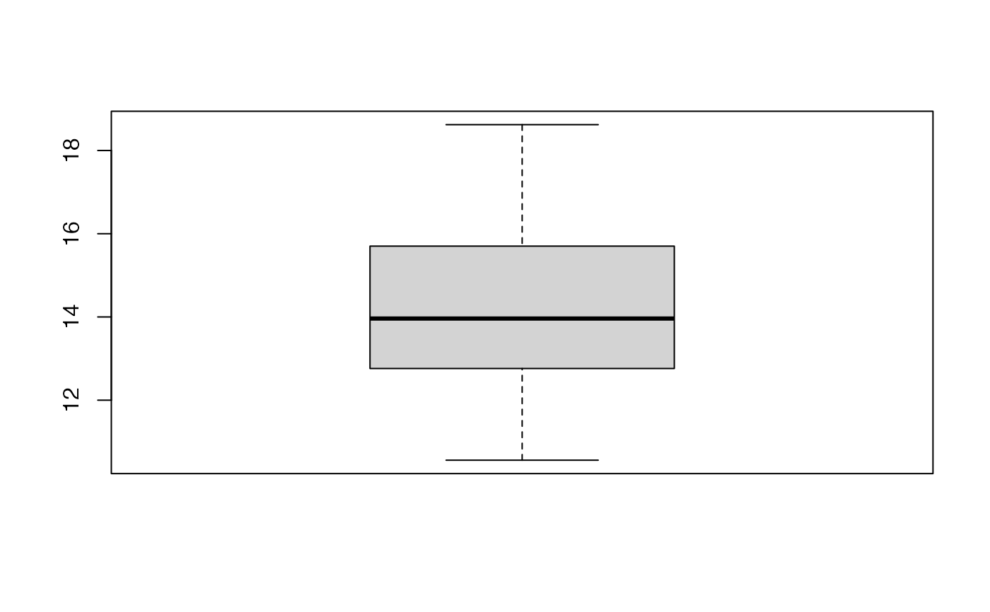 kfolds2Chisqind(bbb2)
#> [[1]]
#> [[1]][[1]]
#> [1] NA NA NA NA NA NA NA NA NA
#>
#> [[1]][[2]]
#> [1] NA NA NA NA NA NA NA NA NA
#>
#> [[1]][[3]]
#> [1] NA NA NA NA NA NA NA NA NA
#>
#> [[1]][[4]]
#> [1] NA NA NA NA NA NA NA NA NA
#>
#> [[1]][[5]]
#> [1] NA NA NA NA NA NA NA NA NA
#>
#> [[1]][[6]]
#> [1] NA NA NA NA NA NA NA NA NA
#>
#> [[1]][[7]]
#> [1] NA NA NA NA NA NA NA NA NA
#>
#> [[1]][[8]]
#> [1] NA NA NA NA NA NA NA NA NA
#>
#> [[1]][[9]]
#> [1] NA NA NA NA NA NA NA NA NA
#>
#> [[1]][[10]]
#> [1] NA NA NA NA NA NA NA NA NA
#>
#>
kfolds2Chisq(bbb2)
#> [[1]]
#> [1] NA NA NA NA NA NA NA NA NA
#>
summary(bbb2)
#> ____************************************************____
#> Only naive DoF can be used with missing data
#>
#> Family: poisson
#> Link function: log
#>
#> ____There are some NAs in X but not in Y____
#> ____Component____ 1 ____
#> ____Component____ 2 ____
#> ____Component____ 3 ____
#> ____Component____ 4 ____
#> ____Component____ 5 ____
#> ____Component____ 6 ____
#> ____Component____ 7 ____
#> ____Component____ 8 ____
#> ____Component____ 9 ____
#> ____Predicting X with NA in X and not in Y____
#> ****________________________________________________****
#>
#>
#> NK: 1
#> [[1]]
#> AIC BIC Q2Chisqcum_Y limQ2 Q2Chisq_Y PREChi2_Pearson_Y
#> Nb_Comp_0 76.61170 78.10821 NA NA NA NA
#> Nb_Comp_1 65.74449 68.73751 NA 0.0975 NA NA
#> Nb_Comp_2 62.35674 66.84626 NA 0.0975 NA NA
#> Nb_Comp_3 62.39804 68.38407 NA 0.0975 NA NA
#> Nb_Comp_4 64.08113 71.56366 NA 0.0975 NA NA
#> Nb_Comp_5 65.63784 74.61689 NA 0.0975 NA NA
#> Nb_Comp_6 67.18468 77.66024 NA 0.0975 NA NA
#> Nb_Comp_7 68.61004 80.58210 NA 0.0975 NA NA
#> Nb_Comp_8 70.54487 84.01344 NA 0.0975 NA NA
#> Nb_Comp_9 72.37296 87.33803 NA 0.0975 NA NA
#> Chi2_Pearson_Y RSS_Y R2_Y
#> Nb_Comp_0 33.75000 24.545455 NA
#> Nb_Comp_1 23.89105 12.654950 0.4844280
#> Nb_Comp_2 17.31172 8.871122 0.6385839
#> Nb_Comp_3 15.51670 8.203709 0.6657748
#> Nb_Comp_4 15.31216 7.959332 0.6757309
#> Nb_Comp_5 15.51159 7.724832 0.6852846
#> Nb_Comp_6 16.30549 6.814620 0.7223673
#> Nb_Comp_7 17.52007 6.284737 0.7439552
#> Nb_Comp_8 17.75766 6.160827 0.7490034
#> Nb_Comp_9 18.30206 5.831059 0.7624383
#>
#> attr(,"class")
#> [1] "summary.cv.plsRglmmodel"
PLS_lm_formula(x11~.,data=pineNAX21,10,typeVC="standard")$InfCrit
#> ____************************************************____
#> Only naive DoF can be used with missing data
#> ____There are some NAs in X but not in Y____
#> ____TypeVC____ standard ____
#> ____TypeVC____ standard ____unknown____
#> ____Component____ 1 ____
#> ____Component____ 2 ____
#> ____Component____ 3 ____
#> ____Component____ 4 ____
#> ____Component____ 5 ____
#> ____Component____ 6 ____
#> ____Component____ 7 ____
#> ____Component____ 8 ____
#> ____Component____ 9 ____
#> Warning : reciprocal condition number of t(cbind(res$pp,temppp)[XXNA[1,],,drop=FALSE])%*%cbind(res$pp,temppp)[XXNA[1,],,drop=FALSE] < 10^{-12}
#> Warning only 9 components could thus be extracted
#> ____Predicting X with NA in X and not in Y____
#> ****________________________________________________****
#>
#> AIC Q2cum_Y LimQ2_Y Q2_Y PRESS_Y RSS_Y
#> Nb_Comp_0 82.41888 NA NA NA NA 20.800152
#> Nb_Comp_1 63.69250 0.35639805 0.0975 0.35639805 13.387018 11.099368
#> Nb_Comp_2 58.35228 0.28395028 0.0975 -0.11256611 12.348781 8.885823
#> Nb_Comp_3 56.36553 0.07664889 0.0975 -0.28950699 11.458331 7.874634
#> Nb_Comp_4 54.02416 -0.70355579 0.0975 -0.84497074 14.528469 6.903925
#> Nb_Comp_5 55.80450 -0.94905654 0.0975 -0.14411078 7.898855 6.858120
#> Nb_Comp_6 57.45753 -1.27568315 0.0975 -0.16758190 8.007417 6.786392
#> Nb_Comp_7 58.73951 -1.63309014 0.0975 -0.15705481 7.852227 6.640327
#> Nb_Comp_8 60.61227 -1.67907859 0.0975 -0.01746558 6.756304 6.614773
#> Nb_Comp_9 62.25948 -2.15165796 0.0975 -0.17639623 7.781594 6.544432
#> R2_Y R2_residY RSS_residY PRESS_residY Q2_residY LimQ2
#> Nb_Comp_0 NA NA 32.00000 NA NA NA
#> Nb_Comp_1 0.4663804 0.4663804 17.07583 20.59526 0.35639805 0.0975
#> Nb_Comp_2 0.5728001 0.5728001 13.67040 18.99799 -0.11256611 0.0975
#> Nb_Comp_3 0.6214146 0.6214146 12.11473 17.62807 -0.28950699 0.0975
#> Nb_Comp_4 0.6680830 0.6680830 10.62135 22.35133 -0.84497074 0.0975
#> Nb_Comp_5 0.6702851 0.6702851 10.55088 12.15200 -0.14411078 0.0975
#> Nb_Comp_6 0.6737336 0.6737336 10.44053 12.31901 -0.16758190 0.0975
#> Nb_Comp_7 0.6807558 0.6807558 10.21581 12.08026 -0.15705481 0.0975
#> Nb_Comp_8 0.6819844 0.6819844 10.17650 10.39424 -0.01746558 0.0975
#> Nb_Comp_9 0.6853661 0.6853661 10.06828 11.97160 -0.17639623 0.0975
#> Q2cum_residY AIC.std DoF.dof sigmahat.dof AIC.dof BIC.dof GMDL.dof
#> Nb_Comp_0 NA 96.63448 NA NA NA NA NA
#> Nb_Comp_1 0.35639805 77.90810 NA NA NA NA NA
#> Nb_Comp_2 0.28395028 72.56787 NA NA NA NA NA
#> Nb_Comp_3 0.07664889 70.58113 NA NA NA NA NA
#> Nb_Comp_4 -0.70355579 68.23976 NA NA NA NA NA
#> Nb_Comp_5 -0.94905654 70.02009 NA NA NA NA NA
#> Nb_Comp_6 -1.27568315 71.67313 NA NA NA NA NA
#> Nb_Comp_7 -1.63309014 72.95511 NA NA NA NA NA
#> Nb_Comp_8 -1.67907859 74.82787 NA NA NA NA NA
#> Nb_Comp_9 -2.15165796 76.47507 NA NA NA NA NA
#> DoF.naive sigmahat.naive AIC.naive BIC.naive GMDL.naive
#> Nb_Comp_0 1 0.8062287 0.6697018 0.6991787 -3.605128
#> Nb_Comp_1 2 0.5983679 0.3797438 0.4122175 -11.413749
#> Nb_Comp_2 3 0.5442372 0.3231208 0.3634169 -12.847656
#> Nb_Comp_3 4 0.5210941 0.3044529 0.3537087 -12.776843
#> Nb_Comp_4 5 0.4965569 0.2839276 0.3398355 -12.891035
#> Nb_Comp_5 6 0.5039885 0.3001871 0.3692997 -11.349498
#> Nb_Comp_6 7 0.5108963 0.3163819 0.3992388 -9.922119
#> Nb_Comp_7 8 0.5153766 0.3300041 0.4263658 -8.696873
#> Nb_Comp_8 9 0.5249910 0.3507834 0.4632727 -7.337679
#> Nb_Comp_9 10 0.5334234 0.3707649 0.4998004 -6.033403
rm(list=c("bbb","bbb2"))
data(pine)
bbb <- cv.plsRglm(x11~.,data=pine,nt=10,modele="pls-glm-family",
family=Gamma,K=10,keepcoeffs=TRUE,keepfolds=FALSE,verbose=FALSE)
#> Warning: NaNs produced
bbb <- cv.plsRglm(x11~.,data=pine,nt=10,modele="pls-glm-Gamma",
K=10,keepcoeffs=TRUE,keepfolds=FALSE,verbose=FALSE)
#For Jackknife computations
kfolds2coeff(bbb)
#> [,1] [,2] [,3] [,4] [,5] [,6]
#> [1,] -16.792342 0.005236079 0.10926655 -0.21333447 2.301769 -0.4448298
#> [2,] -14.234610 0.006332738 0.04999250 -0.27453618 1.891351 -0.3488068
#> [3,] -5.844789 0.007117475 -0.06469022 0.37920549 1.335298 -0.3061289
#> [4,] -9.932799 0.005322613 0.05942021 -0.07160385 2.053345 -0.4252070
#> [5,] -12.774065 0.006741090 0.03326580 -0.17160692 1.876863 -0.3876373
#> [6,] -13.702999 0.006244324 0.03880042 -0.25984490 1.532138 -0.2949647
#> [7,] -14.210322 0.007292974 0.04353365 -0.22707691 1.832913 -0.3381223
#> [8,] -9.939151 0.005128945 0.03243690 -0.09119951 1.710555 -0.3699950
#> [9,] -10.404425 0.004419537 0.03893195 -0.18407583 1.337004 -0.2877251
#> [10,] -11.697334 0.005560470 0.03743670 -0.17084381 1.694513 -0.3408502
#> [,7] [,8] [,9] [,10] [,11]
#> [1,] 2.469793 1.06903574 -0.31839346 1.48350871 0.8169467
#> [2,] 3.828627 -0.67658291 -0.37425278 1.00617016 1.0680206
#> [3,] -3.970980 0.05992600 0.15889027 0.08461725 0.5449955
#> [4,] 0.893972 -0.23958181 -0.19695678 0.60757259 0.3634518
#> [5,] 2.136043 -0.51600999 -0.26135056 1.14341243 0.8057468
#> [6,] 3.153256 -0.46261855 -0.27290448 1.44831281 0.8710504
#> [7,] 3.264836 -0.73899822 -0.36692526 0.96385542 0.8439426
#> [8,] 1.111675 -0.21287594 -0.06494115 0.69672266 0.5415921
#> [9,] 2.212431 0.01529659 -0.06112184 0.96665142 0.3672662
#> [10,] 2.366473 -0.34801334 -0.22585906 0.99273080 0.6957553
boxplot(kfolds2coeff(bbb)[,1])
kfolds2Chisqind(bbb2)
#> [[1]]
#> [[1]][[1]]
#> [1] NA NA NA NA NA NA NA NA NA
#>
#> [[1]][[2]]
#> [1] NA NA NA NA NA NA NA NA NA
#>
#> [[1]][[3]]
#> [1] NA NA NA NA NA NA NA NA NA
#>
#> [[1]][[4]]
#> [1] NA NA NA NA NA NA NA NA NA
#>
#> [[1]][[5]]
#> [1] NA NA NA NA NA NA NA NA NA
#>
#> [[1]][[6]]
#> [1] NA NA NA NA NA NA NA NA NA
#>
#> [[1]][[7]]
#> [1] NA NA NA NA NA NA NA NA NA
#>
#> [[1]][[8]]
#> [1] NA NA NA NA NA NA NA NA NA
#>
#> [[1]][[9]]
#> [1] NA NA NA NA NA NA NA NA NA
#>
#> [[1]][[10]]
#> [1] NA NA NA NA NA NA NA NA NA
#>
#>
kfolds2Chisq(bbb2)
#> [[1]]
#> [1] NA NA NA NA NA NA NA NA NA
#>
summary(bbb2)
#> ____************************************************____
#> Only naive DoF can be used with missing data
#>
#> Family: poisson
#> Link function: log
#>
#> ____There are some NAs in X but not in Y____
#> ____Component____ 1 ____
#> ____Component____ 2 ____
#> ____Component____ 3 ____
#> ____Component____ 4 ____
#> ____Component____ 5 ____
#> ____Component____ 6 ____
#> ____Component____ 7 ____
#> ____Component____ 8 ____
#> ____Component____ 9 ____
#> ____Predicting X with NA in X and not in Y____
#> ****________________________________________________****
#>
#>
#> NK: 1
#> [[1]]
#> AIC BIC Q2Chisqcum_Y limQ2 Q2Chisq_Y PREChi2_Pearson_Y
#> Nb_Comp_0 76.61170 78.10821 NA NA NA NA
#> Nb_Comp_1 65.74449 68.73751 NA 0.0975 NA NA
#> Nb_Comp_2 62.35674 66.84626 NA 0.0975 NA NA
#> Nb_Comp_3 62.39804 68.38407 NA 0.0975 NA NA
#> Nb_Comp_4 64.08113 71.56366 NA 0.0975 NA NA
#> Nb_Comp_5 65.63784 74.61689 NA 0.0975 NA NA
#> Nb_Comp_6 67.18468 77.66024 NA 0.0975 NA NA
#> Nb_Comp_7 68.61004 80.58210 NA 0.0975 NA NA
#> Nb_Comp_8 70.54487 84.01344 NA 0.0975 NA NA
#> Nb_Comp_9 72.37296 87.33803 NA 0.0975 NA NA
#> Chi2_Pearson_Y RSS_Y R2_Y
#> Nb_Comp_0 33.75000 24.545455 NA
#> Nb_Comp_1 23.89105 12.654950 0.4844280
#> Nb_Comp_2 17.31172 8.871122 0.6385839
#> Nb_Comp_3 15.51670 8.203709 0.6657748
#> Nb_Comp_4 15.31216 7.959332 0.6757309
#> Nb_Comp_5 15.51159 7.724832 0.6852846
#> Nb_Comp_6 16.30549 6.814620 0.7223673
#> Nb_Comp_7 17.52007 6.284737 0.7439552
#> Nb_Comp_8 17.75766 6.160827 0.7490034
#> Nb_Comp_9 18.30206 5.831059 0.7624383
#>
#> attr(,"class")
#> [1] "summary.cv.plsRglmmodel"
PLS_lm_formula(x11~.,data=pineNAX21,10,typeVC="standard")$InfCrit
#> ____************************************************____
#> Only naive DoF can be used with missing data
#> ____There are some NAs in X but not in Y____
#> ____TypeVC____ standard ____
#> ____TypeVC____ standard ____unknown____
#> ____Component____ 1 ____
#> ____Component____ 2 ____
#> ____Component____ 3 ____
#> ____Component____ 4 ____
#> ____Component____ 5 ____
#> ____Component____ 6 ____
#> ____Component____ 7 ____
#> ____Component____ 8 ____
#> ____Component____ 9 ____
#> Warning : reciprocal condition number of t(cbind(res$pp,temppp)[XXNA[1,],,drop=FALSE])%*%cbind(res$pp,temppp)[XXNA[1,],,drop=FALSE] < 10^{-12}
#> Warning only 9 components could thus be extracted
#> ____Predicting X with NA in X and not in Y____
#> ****________________________________________________****
#>
#> AIC Q2cum_Y LimQ2_Y Q2_Y PRESS_Y RSS_Y
#> Nb_Comp_0 82.41888 NA NA NA NA 20.800152
#> Nb_Comp_1 63.69250 0.35639805 0.0975 0.35639805 13.387018 11.099368
#> Nb_Comp_2 58.35228 0.28395028 0.0975 -0.11256611 12.348781 8.885823
#> Nb_Comp_3 56.36553 0.07664889 0.0975 -0.28950699 11.458331 7.874634
#> Nb_Comp_4 54.02416 -0.70355579 0.0975 -0.84497074 14.528469 6.903925
#> Nb_Comp_5 55.80450 -0.94905654 0.0975 -0.14411078 7.898855 6.858120
#> Nb_Comp_6 57.45753 -1.27568315 0.0975 -0.16758190 8.007417 6.786392
#> Nb_Comp_7 58.73951 -1.63309014 0.0975 -0.15705481 7.852227 6.640327
#> Nb_Comp_8 60.61227 -1.67907859 0.0975 -0.01746558 6.756304 6.614773
#> Nb_Comp_9 62.25948 -2.15165796 0.0975 -0.17639623 7.781594 6.544432
#> R2_Y R2_residY RSS_residY PRESS_residY Q2_residY LimQ2
#> Nb_Comp_0 NA NA 32.00000 NA NA NA
#> Nb_Comp_1 0.4663804 0.4663804 17.07583 20.59526 0.35639805 0.0975
#> Nb_Comp_2 0.5728001 0.5728001 13.67040 18.99799 -0.11256611 0.0975
#> Nb_Comp_3 0.6214146 0.6214146 12.11473 17.62807 -0.28950699 0.0975
#> Nb_Comp_4 0.6680830 0.6680830 10.62135 22.35133 -0.84497074 0.0975
#> Nb_Comp_5 0.6702851 0.6702851 10.55088 12.15200 -0.14411078 0.0975
#> Nb_Comp_6 0.6737336 0.6737336 10.44053 12.31901 -0.16758190 0.0975
#> Nb_Comp_7 0.6807558 0.6807558 10.21581 12.08026 -0.15705481 0.0975
#> Nb_Comp_8 0.6819844 0.6819844 10.17650 10.39424 -0.01746558 0.0975
#> Nb_Comp_9 0.6853661 0.6853661 10.06828 11.97160 -0.17639623 0.0975
#> Q2cum_residY AIC.std DoF.dof sigmahat.dof AIC.dof BIC.dof GMDL.dof
#> Nb_Comp_0 NA 96.63448 NA NA NA NA NA
#> Nb_Comp_1 0.35639805 77.90810 NA NA NA NA NA
#> Nb_Comp_2 0.28395028 72.56787 NA NA NA NA NA
#> Nb_Comp_3 0.07664889 70.58113 NA NA NA NA NA
#> Nb_Comp_4 -0.70355579 68.23976 NA NA NA NA NA
#> Nb_Comp_5 -0.94905654 70.02009 NA NA NA NA NA
#> Nb_Comp_6 -1.27568315 71.67313 NA NA NA NA NA
#> Nb_Comp_7 -1.63309014 72.95511 NA NA NA NA NA
#> Nb_Comp_8 -1.67907859 74.82787 NA NA NA NA NA
#> Nb_Comp_9 -2.15165796 76.47507 NA NA NA NA NA
#> DoF.naive sigmahat.naive AIC.naive BIC.naive GMDL.naive
#> Nb_Comp_0 1 0.8062287 0.6697018 0.6991787 -3.605128
#> Nb_Comp_1 2 0.5983679 0.3797438 0.4122175 -11.413749
#> Nb_Comp_2 3 0.5442372 0.3231208 0.3634169 -12.847656
#> Nb_Comp_3 4 0.5210941 0.3044529 0.3537087 -12.776843
#> Nb_Comp_4 5 0.4965569 0.2839276 0.3398355 -12.891035
#> Nb_Comp_5 6 0.5039885 0.3001871 0.3692997 -11.349498
#> Nb_Comp_6 7 0.5108963 0.3163819 0.3992388 -9.922119
#> Nb_Comp_7 8 0.5153766 0.3300041 0.4263658 -8.696873
#> Nb_Comp_8 9 0.5249910 0.3507834 0.4632727 -7.337679
#> Nb_Comp_9 10 0.5334234 0.3707649 0.4998004 -6.033403
rm(list=c("bbb","bbb2"))
data(pine)
bbb <- cv.plsRglm(x11~.,data=pine,nt=10,modele="pls-glm-family",
family=Gamma,K=10,keepcoeffs=TRUE,keepfolds=FALSE,verbose=FALSE)
#> Warning: NaNs produced
bbb <- cv.plsRglm(x11~.,data=pine,nt=10,modele="pls-glm-Gamma",
K=10,keepcoeffs=TRUE,keepfolds=FALSE,verbose=FALSE)
#For Jackknife computations
kfolds2coeff(bbb)
#> [,1] [,2] [,3] [,4] [,5] [,6]
#> [1,] -16.792342 0.005236079 0.10926655 -0.21333447 2.301769 -0.4448298
#> [2,] -14.234610 0.006332738 0.04999250 -0.27453618 1.891351 -0.3488068
#> [3,] -5.844789 0.007117475 -0.06469022 0.37920549 1.335298 -0.3061289
#> [4,] -9.932799 0.005322613 0.05942021 -0.07160385 2.053345 -0.4252070
#> [5,] -12.774065 0.006741090 0.03326580 -0.17160692 1.876863 -0.3876373
#> [6,] -13.702999 0.006244324 0.03880042 -0.25984490 1.532138 -0.2949647
#> [7,] -14.210322 0.007292974 0.04353365 -0.22707691 1.832913 -0.3381223
#> [8,] -9.939151 0.005128945 0.03243690 -0.09119951 1.710555 -0.3699950
#> [9,] -10.404425 0.004419537 0.03893195 -0.18407583 1.337004 -0.2877251
#> [10,] -11.697334 0.005560470 0.03743670 -0.17084381 1.694513 -0.3408502
#> [,7] [,8] [,9] [,10] [,11]
#> [1,] 2.469793 1.06903574 -0.31839346 1.48350871 0.8169467
#> [2,] 3.828627 -0.67658291 -0.37425278 1.00617016 1.0680206
#> [3,] -3.970980 0.05992600 0.15889027 0.08461725 0.5449955
#> [4,] 0.893972 -0.23958181 -0.19695678 0.60757259 0.3634518
#> [5,] 2.136043 -0.51600999 -0.26135056 1.14341243 0.8057468
#> [6,] 3.153256 -0.46261855 -0.27290448 1.44831281 0.8710504
#> [7,] 3.264836 -0.73899822 -0.36692526 0.96385542 0.8439426
#> [8,] 1.111675 -0.21287594 -0.06494115 0.69672266 0.5415921
#> [9,] 2.212431 0.01529659 -0.06112184 0.96665142 0.3672662
#> [10,] 2.366473 -0.34801334 -0.22585906 0.99273080 0.6957553
boxplot(kfolds2coeff(bbb)[,1])
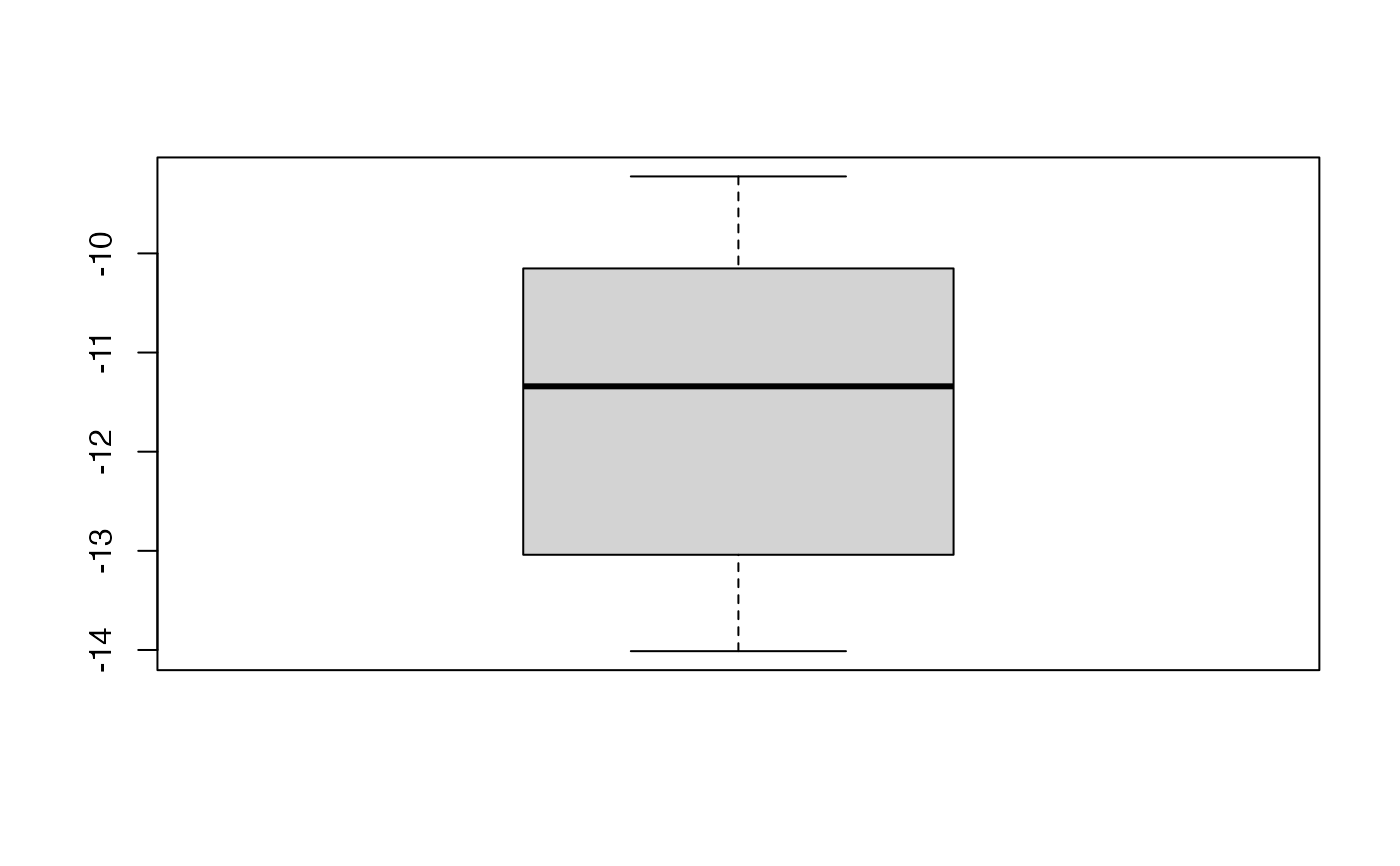 kfolds2Chisqind(bbb)
#> [[1]]
#> [[1]][[1]]
#> [1] NA NA NA NA NA NA NA NA NA NA
#>
#> [[1]][[2]]
#> [1] NA NA NA NA NA NA NA NA NA NA
#>
#> [[1]][[3]]
#> [1] NA NA NA NA NA NA NA NA NA NA
#>
#> [[1]][[4]]
#> [1] NA NA NA NA NA NA NA NA NA NA
#>
#> [[1]][[5]]
#> [1] NA NA NA NA NA NA NA NA NA NA
#>
#> [[1]][[6]]
#> [1] NA NA NA NA NA NA NA NA NA NA
#>
#> [[1]][[7]]
#> [1] NA NA NA NA NA NA NA NA NA NA
#>
#> [[1]][[8]]
#> [1] NA NA NA NA NA NA NA NA NA NA
#>
#> [[1]][[9]]
#> [1] NA NA NA NA NA NA NA NA NA NA
#>
#> [[1]][[10]]
#> [1] NA NA NA NA NA NA NA NA NA NA
#>
#>
kfolds2Chisq(bbb)
#> [[1]]
#> [1] NA NA NA NA NA NA NA NA NA NA
#>
summary(bbb)
#> ____************************************************____
#>
#> Family: Gamma
#> Link function: inverse
#>
#> ____Component____ 1 ____
#> ____Component____ 2 ____
#> ____Component____ 3 ____
#> ____Component____ 4 ____
#> ____Component____ 5 ____
#> ____Component____ 6 ____
#> ____Component____ 7 ____
#> ____Component____ 8 ____
#> ____Component____ 9 ____
#> ____Component____ 10 ____
#> ____Predicting X without NA neither in X or Y____
#> ****________________________________________________****
#>
#>
#> NK: 1
#> [[1]]
#> AIC BIC Q2Chisqcum_Y limQ2 Q2Chisq_Y PREChi2_Pearson_Y
#> Nb_Comp_0 56.60919 59.60220 NA NA NA NA
#> Nb_Comp_1 39.01090 43.50042 NA 0.0975 NA NA
#> Nb_Comp_2 37.30801 43.29404 NA 0.0975 NA NA
#> Nb_Comp_3 36.87524 44.35777 NA 0.0975 NA NA
#> Nb_Comp_4 36.55795 45.53700 NA 0.0975 NA NA
#> Nb_Comp_5 37.13611 47.61167 NA 0.0975 NA NA
#> Nb_Comp_6 38.27656 50.24862 NA 0.0975 NA NA
#> Nb_Comp_7 39.39377 52.86234 NA 0.0975 NA NA
#> Nb_Comp_8 40.96122 55.92630 NA 0.0975 NA NA
#> Nb_Comp_9 42.90816 59.36974 NA 0.0975 NA NA
#> Nb_Comp_10 44.90815 62.86625 NA 0.0975 NA NA
#> Chi2_Pearson_Y RSS_Y R2_Y
#> Nb_Comp_0 31.60805 20.800152 NA
#> Nb_Comp_1 17.31431 11.804594 0.4324756
#> Nb_Comp_2 17.01037 6.357437 0.6943562
#> Nb_Comp_3 15.83422 5.699662 0.7259798
#> Nb_Comp_4 13.52676 7.679741 0.6307844
#> Nb_Comp_5 13.60962 6.099077 0.7067773
#> Nb_Comp_6 13.91155 5.205052 0.7497590
#> Nb_Comp_7 14.94390 4.650377 0.7764258
#> Nb_Comp_8 15.25537 4.321314 0.7922461
#> Nb_Comp_9 15.15577 4.307757 0.7928978
#> Nb_Comp_10 15.15490 4.307391 0.7929154
#>
#> attr(,"class")
#> [1] "summary.cv.plsRglmmodel"
PLS_lm_formula(x11~.,data=pine,10,typeVC="standard")$InfCrit
#> ____************************************************____
#> ____TypeVC____ standard ____
#> ____Component____ 1 ____
#> ____Component____ 2 ____
#> ____Component____ 3 ____
#> ____Component____ 4 ____
#> ____Component____ 5 ____
#> ____Component____ 6 ____
#> ____Component____ 7 ____
#> ____Component____ 8 ____
#> ____Component____ 9 ____
#> ____Component____ 10 ____
#> ____Predicting X without NA neither in X nor in Y____
#> ****________________________________________________****
#>
#> AIC Q2cum_Y LimQ2_Y Q2_Y PRESS_Y RSS_Y
#> Nb_Comp_0 82.41888 NA NA NA NA 20.800152
#> Nb_Comp_1 63.61896 0.38248575 0.0975 0.38248575 12.844390 11.074659
#> Nb_Comp_2 58.47638 0.34836456 0.0975 -0.05525570 11.686597 8.919303
#> Nb_Comp_3 56.55421 0.23688359 0.0975 -0.17107874 10.445206 7.919786
#> Nb_Comp_4 54.35053 0.06999681 0.0975 -0.21869112 9.651773 6.972542
#> Nb_Comp_5 55.99834 -0.07691053 0.0975 -0.15796434 8.073955 6.898523
#> Nb_Comp_6 57.69592 -0.19968885 0.0975 -0.11400977 7.685022 6.835594
#> Nb_Comp_7 59.37953 -0.27722139 0.0975 -0.06462721 7.277359 6.770369
#> Nb_Comp_8 61.21213 -0.30602578 0.0975 -0.02255238 6.923057 6.736112
#> Nb_Comp_9 63.18426 -0.39920228 0.0975 -0.07134354 7.216690 6.730426
#> Nb_Comp_10 65.15982 -0.43743644 0.0975 -0.02732569 6.914340 6.725443
#> R2_Y R2_residY RSS_residY PRESS_residY Q2_residY LimQ2
#> Nb_Comp_0 NA NA 32.00000 NA NA NA
#> Nb_Comp_1 0.4675684 0.4675684 17.03781 19.76046 0.38248575 0.0975
#> Nb_Comp_2 0.5711905 0.5711905 13.72190 17.97925 -0.05525570 0.0975
#> Nb_Comp_3 0.6192438 0.6192438 12.18420 16.06943 -0.17107874 0.0975
#> Nb_Comp_4 0.6647841 0.6647841 10.72691 14.84877 -0.21869112 0.0975
#> Nb_Comp_5 0.6683426 0.6683426 10.61304 12.42138 -0.15796434 0.0975
#> Nb_Comp_6 0.6713681 0.6713681 10.51622 11.82303 -0.11400977 0.0975
#> Nb_Comp_7 0.6745039 0.6745039 10.41588 11.19586 -0.06462721 0.0975
#> Nb_Comp_8 0.6761508 0.6761508 10.36317 10.65078 -0.02255238 0.0975
#> Nb_Comp_9 0.6764242 0.6764242 10.35443 11.10252 -0.07134354 0.0975
#> Nb_Comp_10 0.6766638 0.6766638 10.34676 10.63737 -0.02732569 0.0975
#> Q2cum_residY AIC.std DoF.dof sigmahat.dof AIC.dof BIC.dof
#> Nb_Comp_0 NA 96.63448 1.000000 0.8062287 0.6697018 0.6991787
#> Nb_Comp_1 0.38248575 77.83455 3.176360 0.5994089 0.4047616 0.4565153
#> Nb_Comp_2 0.34836456 72.69198 7.133559 0.5761829 0.4138120 0.5212090
#> Nb_Comp_3 0.23688359 70.76981 8.778329 0.5603634 0.4070516 0.5320535
#> Nb_Comp_4 0.06999681 68.56612 8.427874 0.5221703 0.3505594 0.4547689
#> Nb_Comp_5 -0.07691053 70.21393 9.308247 0.5285695 0.3666578 0.4845912
#> Nb_Comp_6 -0.19968885 71.91152 9.291931 0.5259794 0.3629363 0.4795121
#> Nb_Comp_7 -0.27722139 73.59512 9.756305 0.5284535 0.3702885 0.4938445
#> Nb_Comp_8 -0.30602578 75.42772 10.363948 0.5338475 0.3831339 0.5170783
#> Nb_Comp_9 -0.39920228 77.39986 10.732146 0.5378276 0.3920957 0.5328746
#> Nb_Comp_10 -0.43743644 79.37542 11.000000 0.5407500 0.3987417 0.5446065
#> GMDL.dof DoF.naive sigmahat.naive AIC.naive BIC.naive GMDL.naive
#> Nb_Comp_0 -3.605128 1 0.8062287 0.6697018 0.6991787 -3.605128
#> Nb_Comp_1 -9.875081 2 0.5977015 0.3788984 0.4112998 -11.451340
#> Nb_Comp_2 -6.985517 3 0.5452615 0.3243383 0.3647862 -12.822703
#> Nb_Comp_3 -6.260610 4 0.5225859 0.3061986 0.3557368 -12.756838
#> Nb_Comp_4 -8.152986 5 0.4990184 0.2867496 0.3432131 -12.811575
#> Nb_Comp_5 -7.111583 6 0.5054709 0.3019556 0.3714754 -11.329638
#> Nb_Comp_6 -7.233043 7 0.5127450 0.3186757 0.4021333 -9.918688
#> Nb_Comp_7 -6.742195 8 0.5203986 0.3364668 0.4347156 -8.592770
#> Nb_Comp_8 -6.038372 9 0.5297842 0.3572181 0.4717708 -7.287834
#> Nb_Comp_9 -5.600237 10 0.5409503 0.3813021 0.5140048 -6.008747
#> Nb_Comp_10 -5.288422 11 0.5529032 0.4076026 0.5600977 -4.799453
data(pineNAX21)
bbb2 <- cv.plsRglm(x11~.,data=pineNAX21,nt=10,
modele="pls-glm-family",family=Gamma(),K=10,keepcoeffs=TRUE,keepfolds=FALSE,verbose=FALSE)
#> Warning: NaNs produced
#> Warning: NaNs produced
#> Warning: NaNs produced
bbb2 <- cv.plsRglm(x11~.,data=pineNAX21,nt=10,
modele="pls-glm-Gamma",K=10,keepcoeffs=TRUE,keepfolds=FALSE,verbose=FALSE)
#For Jackknife computations
kfolds2coeff(bbb2)
#> [,1] [,2] [,3] [,4] [,5] [,6]
#> [1,] -21.14485 0.008616130 0.03674745 -0.3581602 1.921926 -0.4081026
#> [2,] -14.59880 0.006080550 0.04715798 -0.2438525 1.489233 -0.2797521
#> [3,] -18.91294 0.006700005 0.01866432 -0.3322595 2.532909 -0.4118893
#> [4,] -12.67608 0.009417885 -0.01566997 0.2352732 1.859993 -0.3336438
#> [5,] -13.34389 0.004652787 0.07361635 -0.1620116 2.834521 -0.5773882
#> [6,] -13.17192 0.005094255 0.04154328 -0.1750301 1.509127 -0.3823807
#> [7,] -14.64076 0.005851807 0.04253858 -0.1765887 1.619940 -0.3502596
#> [8,] -14.05079 0.006416756 0.04498837 -0.1547725 1.853500 -0.3772898
#> [9,] -14.81978 0.005565971 0.03091156 -0.2176143 1.414826 -0.2538928
#> [10,] -16.70714 0.006712930 0.05073523 -0.2151543 2.071076 -0.4216196
#> [,7] [,8] [,9] [,10] [,11]
#> [1,] 5.085774 -1.20930485 -0.11055368 -0.08804458 2.4880806
#> [2,] 3.129944 0.44686098 -0.34791666 1.35572433 0.7578715
#> [3,] 4.666129 -1.54297343 -0.47202093 0.90615274 2.4111899
#> [4,] -2.131302 -0.64364488 -0.40458513 0.81511245 0.7576426
#> [5,] 2.318833 -0.91278561 -0.28582585 0.48299052 1.0030298
#> [6,] 1.722917 0.35048599 0.04318401 1.14731994 0.0239185
#> [7,] 2.522483 -0.06485633 -0.15403482 0.62898504 0.7546944
#> [8,] 2.363459 -0.65334098 -0.21317757 0.36778230 0.7469297
#> [9,] 2.547778 0.02973721 -0.22484351 1.55589269 0.3409361
#> [10,] 2.939051 -0.48799520 -0.26474681 0.85336920 1.1093337
boxplot(kfolds2coeff(bbb2)[,1])
kfolds2Chisqind(bbb)
#> [[1]]
#> [[1]][[1]]
#> [1] NA NA NA NA NA NA NA NA NA NA
#>
#> [[1]][[2]]
#> [1] NA NA NA NA NA NA NA NA NA NA
#>
#> [[1]][[3]]
#> [1] NA NA NA NA NA NA NA NA NA NA
#>
#> [[1]][[4]]
#> [1] NA NA NA NA NA NA NA NA NA NA
#>
#> [[1]][[5]]
#> [1] NA NA NA NA NA NA NA NA NA NA
#>
#> [[1]][[6]]
#> [1] NA NA NA NA NA NA NA NA NA NA
#>
#> [[1]][[7]]
#> [1] NA NA NA NA NA NA NA NA NA NA
#>
#> [[1]][[8]]
#> [1] NA NA NA NA NA NA NA NA NA NA
#>
#> [[1]][[9]]
#> [1] NA NA NA NA NA NA NA NA NA NA
#>
#> [[1]][[10]]
#> [1] NA NA NA NA NA NA NA NA NA NA
#>
#>
kfolds2Chisq(bbb)
#> [[1]]
#> [1] NA NA NA NA NA NA NA NA NA NA
#>
summary(bbb)
#> ____************************************************____
#>
#> Family: Gamma
#> Link function: inverse
#>
#> ____Component____ 1 ____
#> ____Component____ 2 ____
#> ____Component____ 3 ____
#> ____Component____ 4 ____
#> ____Component____ 5 ____
#> ____Component____ 6 ____
#> ____Component____ 7 ____
#> ____Component____ 8 ____
#> ____Component____ 9 ____
#> ____Component____ 10 ____
#> ____Predicting X without NA neither in X or Y____
#> ****________________________________________________****
#>
#>
#> NK: 1
#> [[1]]
#> AIC BIC Q2Chisqcum_Y limQ2 Q2Chisq_Y PREChi2_Pearson_Y
#> Nb_Comp_0 56.60919 59.60220 NA NA NA NA
#> Nb_Comp_1 39.01090 43.50042 NA 0.0975 NA NA
#> Nb_Comp_2 37.30801 43.29404 NA 0.0975 NA NA
#> Nb_Comp_3 36.87524 44.35777 NA 0.0975 NA NA
#> Nb_Comp_4 36.55795 45.53700 NA 0.0975 NA NA
#> Nb_Comp_5 37.13611 47.61167 NA 0.0975 NA NA
#> Nb_Comp_6 38.27656 50.24862 NA 0.0975 NA NA
#> Nb_Comp_7 39.39377 52.86234 NA 0.0975 NA NA
#> Nb_Comp_8 40.96122 55.92630 NA 0.0975 NA NA
#> Nb_Comp_9 42.90816 59.36974 NA 0.0975 NA NA
#> Nb_Comp_10 44.90815 62.86625 NA 0.0975 NA NA
#> Chi2_Pearson_Y RSS_Y R2_Y
#> Nb_Comp_0 31.60805 20.800152 NA
#> Nb_Comp_1 17.31431 11.804594 0.4324756
#> Nb_Comp_2 17.01037 6.357437 0.6943562
#> Nb_Comp_3 15.83422 5.699662 0.7259798
#> Nb_Comp_4 13.52676 7.679741 0.6307844
#> Nb_Comp_5 13.60962 6.099077 0.7067773
#> Nb_Comp_6 13.91155 5.205052 0.7497590
#> Nb_Comp_7 14.94390 4.650377 0.7764258
#> Nb_Comp_8 15.25537 4.321314 0.7922461
#> Nb_Comp_9 15.15577 4.307757 0.7928978
#> Nb_Comp_10 15.15490 4.307391 0.7929154
#>
#> attr(,"class")
#> [1] "summary.cv.plsRglmmodel"
PLS_lm_formula(x11~.,data=pine,10,typeVC="standard")$InfCrit
#> ____************************************************____
#> ____TypeVC____ standard ____
#> ____Component____ 1 ____
#> ____Component____ 2 ____
#> ____Component____ 3 ____
#> ____Component____ 4 ____
#> ____Component____ 5 ____
#> ____Component____ 6 ____
#> ____Component____ 7 ____
#> ____Component____ 8 ____
#> ____Component____ 9 ____
#> ____Component____ 10 ____
#> ____Predicting X without NA neither in X nor in Y____
#> ****________________________________________________****
#>
#> AIC Q2cum_Y LimQ2_Y Q2_Y PRESS_Y RSS_Y
#> Nb_Comp_0 82.41888 NA NA NA NA 20.800152
#> Nb_Comp_1 63.61896 0.38248575 0.0975 0.38248575 12.844390 11.074659
#> Nb_Comp_2 58.47638 0.34836456 0.0975 -0.05525570 11.686597 8.919303
#> Nb_Comp_3 56.55421 0.23688359 0.0975 -0.17107874 10.445206 7.919786
#> Nb_Comp_4 54.35053 0.06999681 0.0975 -0.21869112 9.651773 6.972542
#> Nb_Comp_5 55.99834 -0.07691053 0.0975 -0.15796434 8.073955 6.898523
#> Nb_Comp_6 57.69592 -0.19968885 0.0975 -0.11400977 7.685022 6.835594
#> Nb_Comp_7 59.37953 -0.27722139 0.0975 -0.06462721 7.277359 6.770369
#> Nb_Comp_8 61.21213 -0.30602578 0.0975 -0.02255238 6.923057 6.736112
#> Nb_Comp_9 63.18426 -0.39920228 0.0975 -0.07134354 7.216690 6.730426
#> Nb_Comp_10 65.15982 -0.43743644 0.0975 -0.02732569 6.914340 6.725443
#> R2_Y R2_residY RSS_residY PRESS_residY Q2_residY LimQ2
#> Nb_Comp_0 NA NA 32.00000 NA NA NA
#> Nb_Comp_1 0.4675684 0.4675684 17.03781 19.76046 0.38248575 0.0975
#> Nb_Comp_2 0.5711905 0.5711905 13.72190 17.97925 -0.05525570 0.0975
#> Nb_Comp_3 0.6192438 0.6192438 12.18420 16.06943 -0.17107874 0.0975
#> Nb_Comp_4 0.6647841 0.6647841 10.72691 14.84877 -0.21869112 0.0975
#> Nb_Comp_5 0.6683426 0.6683426 10.61304 12.42138 -0.15796434 0.0975
#> Nb_Comp_6 0.6713681 0.6713681 10.51622 11.82303 -0.11400977 0.0975
#> Nb_Comp_7 0.6745039 0.6745039 10.41588 11.19586 -0.06462721 0.0975
#> Nb_Comp_8 0.6761508 0.6761508 10.36317 10.65078 -0.02255238 0.0975
#> Nb_Comp_9 0.6764242 0.6764242 10.35443 11.10252 -0.07134354 0.0975
#> Nb_Comp_10 0.6766638 0.6766638 10.34676 10.63737 -0.02732569 0.0975
#> Q2cum_residY AIC.std DoF.dof sigmahat.dof AIC.dof BIC.dof
#> Nb_Comp_0 NA 96.63448 1.000000 0.8062287 0.6697018 0.6991787
#> Nb_Comp_1 0.38248575 77.83455 3.176360 0.5994089 0.4047616 0.4565153
#> Nb_Comp_2 0.34836456 72.69198 7.133559 0.5761829 0.4138120 0.5212090
#> Nb_Comp_3 0.23688359 70.76981 8.778329 0.5603634 0.4070516 0.5320535
#> Nb_Comp_4 0.06999681 68.56612 8.427874 0.5221703 0.3505594 0.4547689
#> Nb_Comp_5 -0.07691053 70.21393 9.308247 0.5285695 0.3666578 0.4845912
#> Nb_Comp_6 -0.19968885 71.91152 9.291931 0.5259794 0.3629363 0.4795121
#> Nb_Comp_7 -0.27722139 73.59512 9.756305 0.5284535 0.3702885 0.4938445
#> Nb_Comp_8 -0.30602578 75.42772 10.363948 0.5338475 0.3831339 0.5170783
#> Nb_Comp_9 -0.39920228 77.39986 10.732146 0.5378276 0.3920957 0.5328746
#> Nb_Comp_10 -0.43743644 79.37542 11.000000 0.5407500 0.3987417 0.5446065
#> GMDL.dof DoF.naive sigmahat.naive AIC.naive BIC.naive GMDL.naive
#> Nb_Comp_0 -3.605128 1 0.8062287 0.6697018 0.6991787 -3.605128
#> Nb_Comp_1 -9.875081 2 0.5977015 0.3788984 0.4112998 -11.451340
#> Nb_Comp_2 -6.985517 3 0.5452615 0.3243383 0.3647862 -12.822703
#> Nb_Comp_3 -6.260610 4 0.5225859 0.3061986 0.3557368 -12.756838
#> Nb_Comp_4 -8.152986 5 0.4990184 0.2867496 0.3432131 -12.811575
#> Nb_Comp_5 -7.111583 6 0.5054709 0.3019556 0.3714754 -11.329638
#> Nb_Comp_6 -7.233043 7 0.5127450 0.3186757 0.4021333 -9.918688
#> Nb_Comp_7 -6.742195 8 0.5203986 0.3364668 0.4347156 -8.592770
#> Nb_Comp_8 -6.038372 9 0.5297842 0.3572181 0.4717708 -7.287834
#> Nb_Comp_9 -5.600237 10 0.5409503 0.3813021 0.5140048 -6.008747
#> Nb_Comp_10 -5.288422 11 0.5529032 0.4076026 0.5600977 -4.799453
data(pineNAX21)
bbb2 <- cv.plsRglm(x11~.,data=pineNAX21,nt=10,
modele="pls-glm-family",family=Gamma(),K=10,keepcoeffs=TRUE,keepfolds=FALSE,verbose=FALSE)
#> Warning: NaNs produced
#> Warning: NaNs produced
#> Warning: NaNs produced
bbb2 <- cv.plsRglm(x11~.,data=pineNAX21,nt=10,
modele="pls-glm-Gamma",K=10,keepcoeffs=TRUE,keepfolds=FALSE,verbose=FALSE)
#For Jackknife computations
kfolds2coeff(bbb2)
#> [,1] [,2] [,3] [,4] [,5] [,6]
#> [1,] -21.14485 0.008616130 0.03674745 -0.3581602 1.921926 -0.4081026
#> [2,] -14.59880 0.006080550 0.04715798 -0.2438525 1.489233 -0.2797521
#> [3,] -18.91294 0.006700005 0.01866432 -0.3322595 2.532909 -0.4118893
#> [4,] -12.67608 0.009417885 -0.01566997 0.2352732 1.859993 -0.3336438
#> [5,] -13.34389 0.004652787 0.07361635 -0.1620116 2.834521 -0.5773882
#> [6,] -13.17192 0.005094255 0.04154328 -0.1750301 1.509127 -0.3823807
#> [7,] -14.64076 0.005851807 0.04253858 -0.1765887 1.619940 -0.3502596
#> [8,] -14.05079 0.006416756 0.04498837 -0.1547725 1.853500 -0.3772898
#> [9,] -14.81978 0.005565971 0.03091156 -0.2176143 1.414826 -0.2538928
#> [10,] -16.70714 0.006712930 0.05073523 -0.2151543 2.071076 -0.4216196
#> [,7] [,8] [,9] [,10] [,11]
#> [1,] 5.085774 -1.20930485 -0.11055368 -0.08804458 2.4880806
#> [2,] 3.129944 0.44686098 -0.34791666 1.35572433 0.7578715
#> [3,] 4.666129 -1.54297343 -0.47202093 0.90615274 2.4111899
#> [4,] -2.131302 -0.64364488 -0.40458513 0.81511245 0.7576426
#> [5,] 2.318833 -0.91278561 -0.28582585 0.48299052 1.0030298
#> [6,] 1.722917 0.35048599 0.04318401 1.14731994 0.0239185
#> [7,] 2.522483 -0.06485633 -0.15403482 0.62898504 0.7546944
#> [8,] 2.363459 -0.65334098 -0.21317757 0.36778230 0.7469297
#> [9,] 2.547778 0.02973721 -0.22484351 1.55589269 0.3409361
#> [10,] 2.939051 -0.48799520 -0.26474681 0.85336920 1.1093337
boxplot(kfolds2coeff(bbb2)[,1])
 kfolds2Chisqind(bbb2)
#> [[1]]
#> [[1]][[1]]
#> [1] NA NA NA NA NA NA NA NA NA
#>
#> [[1]][[2]]
#> [1] NA NA NA NA NA NA NA NA NA
#>
#> [[1]][[3]]
#> [1] NA NA NA NA NA NA NA NA NA
#>
#> [[1]][[4]]
#> [1] NA NA NA NA NA NA NA NA NA
#>
#> [[1]][[5]]
#> [1] NA NA NA NA NA NA NA NA NA
#>
#> [[1]][[6]]
#> [1] NA NA NA NA NA NA NA NA NA
#>
#> [[1]][[7]]
#> [1] NA NA NA NA NA NA NA NA NA
#>
#> [[1]][[8]]
#> [1] NA NA NA NA NA NA NA NA NA
#>
#> [[1]][[9]]
#> [1] NA NA NA NA NA NA NA NA NA
#>
#> [[1]][[10]]
#> [1] NA NA NA NA NA NA NA NA NA
#>
#>
kfolds2Chisq(bbb2)
#> [[1]]
#> [1] NA NA NA NA NA NA NA NA NA
#>
summary(bbb2)
#> ____************************************************____
#> Only naive DoF can be used with missing data
#>
#> Family: Gamma
#> Link function: inverse
#>
#> ____There are some NAs in X but not in Y____
#> ____Component____ 1 ____
#> ____Component____ 2 ____
#> ____Component____ 3 ____
#> ____Component____ 4 ____
#> ____Component____ 5 ____
#> ____Component____ 6 ____
#> ____Component____ 7 ____
#> ____Component____ 8 ____
#> ____Component____ 9 ____
#> ____Predicting X with NA in X and not in Y____
#> ****________________________________________________****
#>
#>
#> NK: 1
#> [[1]]
#> AIC BIC Q2Chisqcum_Y limQ2 Q2Chisq_Y PREChi2_Pearson_Y
#> Nb_Comp_0 56.60919 59.60220 NA NA NA NA
#> Nb_Comp_1 39.08940 43.57892 NA 0.0975 NA NA
#> Nb_Comp_2 37.36154 43.34757 NA 0.0975 NA NA
#> Nb_Comp_3 36.81173 44.29427 NA 0.0975 NA NA
#> Nb_Comp_4 36.53654 45.51559 NA 0.0975 NA NA
#> Nb_Comp_5 37.24312 47.71867 NA 0.0975 NA NA
#> Nb_Comp_6 38.18649 50.15855 NA 0.0975 NA NA
#> Nb_Comp_7 39.35575 52.82432 NA 0.0975 NA NA
#> Nb_Comp_8 40.86209 55.82716 NA 0.0975 NA NA
#> Nb_Comp_9 42.80511 59.26669 NA 0.0975 NA NA
#> Chi2_Pearson_Y RSS_Y R2_Y
#> Nb_Comp_0 31.60805 20.800152 NA
#> Nb_Comp_1 17.30890 12.031518 0.4215659
#> Nb_Comp_2 17.10360 6.183372 0.7027247
#> Nb_Comp_3 15.78579 5.756462 0.7232490
#> Nb_Comp_4 13.49013 7.630460 0.6331536
#> Nb_Comp_5 13.56918 6.303455 0.6969515
#> Nb_Comp_6 14.02295 5.274716 0.7464097
#> Nb_Comp_7 15.05896 4.867806 0.7659726
#> Nb_Comp_8 15.28052 4.317488 0.7924300
#> Nb_Comp_9 15.19429 4.298593 0.7933384
#>
#> attr(,"class")
#> [1] "summary.cv.plsRglmmodel"
PLS_lm_formula(x11~.,data=pineNAX21,10,typeVC="standard")$InfCrit
#> ____************************************************____
#> Only naive DoF can be used with missing data
#> ____There are some NAs in X but not in Y____
#> ____TypeVC____ standard ____
#> ____TypeVC____ standard ____unknown____
#> ____Component____ 1 ____
#> ____Component____ 2 ____
#> ____Component____ 3 ____
#> ____Component____ 4 ____
#> ____Component____ 5 ____
#> ____Component____ 6 ____
#> ____Component____ 7 ____
#> ____Component____ 8 ____
#> ____Component____ 9 ____
#> Warning : reciprocal condition number of t(cbind(res$pp,temppp)[XXNA[1,],,drop=FALSE])%*%cbind(res$pp,temppp)[XXNA[1,],,drop=FALSE] < 10^{-12}
#> Warning only 9 components could thus be extracted
#> ____Predicting X with NA in X and not in Y____
#> ****________________________________________________****
#>
#> AIC Q2cum_Y LimQ2_Y Q2_Y PRESS_Y RSS_Y
#> Nb_Comp_0 82.41888 NA NA NA NA 20.800152
#> Nb_Comp_1 63.69250 0.35639805 0.0975 0.35639805 13.387018 11.099368
#> Nb_Comp_2 58.35228 0.28395028 0.0975 -0.11256611 12.348781 8.885823
#> Nb_Comp_3 56.36553 0.07664889 0.0975 -0.28950699 11.458331 7.874634
#> Nb_Comp_4 54.02416 -0.70355579 0.0975 -0.84497074 14.528469 6.903925
#> Nb_Comp_5 55.80450 -0.94905654 0.0975 -0.14411078 7.898855 6.858120
#> Nb_Comp_6 57.45753 -1.27568315 0.0975 -0.16758190 8.007417 6.786392
#> Nb_Comp_7 58.73951 -1.63309014 0.0975 -0.15705481 7.852227 6.640327
#> Nb_Comp_8 60.61227 -1.67907859 0.0975 -0.01746558 6.756304 6.614773
#> Nb_Comp_9 62.25948 -2.15165796 0.0975 -0.17639623 7.781594 6.544432
#> R2_Y R2_residY RSS_residY PRESS_residY Q2_residY LimQ2
#> Nb_Comp_0 NA NA 32.00000 NA NA NA
#> Nb_Comp_1 0.4663804 0.4663804 17.07583 20.59526 0.35639805 0.0975
#> Nb_Comp_2 0.5728001 0.5728001 13.67040 18.99799 -0.11256611 0.0975
#> Nb_Comp_3 0.6214146 0.6214146 12.11473 17.62807 -0.28950699 0.0975
#> Nb_Comp_4 0.6680830 0.6680830 10.62135 22.35133 -0.84497074 0.0975
#> Nb_Comp_5 0.6702851 0.6702851 10.55088 12.15200 -0.14411078 0.0975
#> Nb_Comp_6 0.6737336 0.6737336 10.44053 12.31901 -0.16758190 0.0975
#> Nb_Comp_7 0.6807558 0.6807558 10.21581 12.08026 -0.15705481 0.0975
#> Nb_Comp_8 0.6819844 0.6819844 10.17650 10.39424 -0.01746558 0.0975
#> Nb_Comp_9 0.6853661 0.6853661 10.06828 11.97160 -0.17639623 0.0975
#> Q2cum_residY AIC.std DoF.dof sigmahat.dof AIC.dof BIC.dof GMDL.dof
#> Nb_Comp_0 NA 96.63448 NA NA NA NA NA
#> Nb_Comp_1 0.35639805 77.90810 NA NA NA NA NA
#> Nb_Comp_2 0.28395028 72.56787 NA NA NA NA NA
#> Nb_Comp_3 0.07664889 70.58113 NA NA NA NA NA
#> Nb_Comp_4 -0.70355579 68.23976 NA NA NA NA NA
#> Nb_Comp_5 -0.94905654 70.02009 NA NA NA NA NA
#> Nb_Comp_6 -1.27568315 71.67313 NA NA NA NA NA
#> Nb_Comp_7 -1.63309014 72.95511 NA NA NA NA NA
#> Nb_Comp_8 -1.67907859 74.82787 NA NA NA NA NA
#> Nb_Comp_9 -2.15165796 76.47507 NA NA NA NA NA
#> DoF.naive sigmahat.naive AIC.naive BIC.naive GMDL.naive
#> Nb_Comp_0 1 0.8062287 0.6697018 0.6991787 -3.605128
#> Nb_Comp_1 2 0.5983679 0.3797438 0.4122175 -11.413749
#> Nb_Comp_2 3 0.5442372 0.3231208 0.3634169 -12.847656
#> Nb_Comp_3 4 0.5210941 0.3044529 0.3537087 -12.776843
#> Nb_Comp_4 5 0.4965569 0.2839276 0.3398355 -12.891035
#> Nb_Comp_5 6 0.5039885 0.3001871 0.3692997 -11.349498
#> Nb_Comp_6 7 0.5108963 0.3163819 0.3992388 -9.922119
#> Nb_Comp_7 8 0.5153766 0.3300041 0.4263658 -8.696873
#> Nb_Comp_8 9 0.5249910 0.3507834 0.4632727 -7.337679
#> Nb_Comp_9 10 0.5334234 0.3707649 0.4998004 -6.033403
rm(list=c("bbb","bbb2"))
data(Cornell)
summary(cv.plsRglm(Y~.,data=Cornell,nt=10,NK=1,modele="pls",verbose=FALSE))
#> ____************************************************____
#>
#> Model: pls
#>
#> ____Component____ 1 ____
#> ____Component____ 2 ____
#> ____Component____ 3 ____
#> ____Component____ 4 ____
#> ____Component____ 5 ____
#> ____Component____ 6 ____
#> ____Predicting X without NA neither in X or Y____
#> ****________________________________________________****
#>
#>
#> NK: 1
#> [[1]]
#> AIC Q2cum_Y LimQ2_Y Q2_Y PRESS_Y RSS_Y R2_Y
#> Nb_Comp_0 82.01205 NA NA NA NA 467.796667 NA
#> Nb_Comp_1 53.15173 0.8909588 0.0975 0.8909588 51.00912 35.742486 0.9235940
#> Nb_Comp_2 41.08283 0.8463898 0.0975 -0.4087353 50.35170 11.066606 0.9763431
#> Nb_Comp_3 32.06411 0.5671404 0.0975 -1.8179088 31.18469 4.418081 0.9905556
#> Nb_Comp_4 33.76477 -0.7046676 0.0975 -2.9381536 17.39908 4.309235 0.9907882
#> Nb_Comp_5 33.34373 -5.1246265 0.0975 -2.5928569 15.48247 3.521924 0.9924713
#> Nb_Comp_6 35.25533 NA 0.0975 NA NA 3.496074 0.9925265
#> AIC.std DoF.dof sigmahat.dof AIC.dof BIC.dof GMDL.dof
#> Nb_Comp_0 37.010388 1.000000 6.5212706 46.0708838 47.7893514 27.59461
#> Nb_Comp_1 8.150064 2.740749 1.8665281 4.5699686 4.9558156 21.34020
#> Nb_Comp_2 -3.918831 5.085967 1.1825195 2.1075461 2.3949331 27.40202
#> Nb_Comp_3 -12.937550 5.121086 0.7488308 0.8467795 0.9628191 24.40842
#> Nb_Comp_4 -11.236891 5.103312 0.7387162 0.8232505 0.9357846 24.23105
#> Nb_Comp_5 -11.657929 6.006316 0.7096382 0.7976101 0.9198348 28.21184
#> Nb_Comp_6 -9.746328 7.000002 0.7633343 0.9711321 1.1359501 33.18347
#> DoF.naive sigmahat.naive AIC.naive BIC.naive GMDL.naive
#> Nb_Comp_0 1 6.5212706 46.0708838 47.7893514 27.59461
#> Nb_Comp_1 2 1.8905683 4.1699567 4.4588195 18.37545
#> Nb_Comp_2 3 1.1088836 1.5370286 1.6860917 17.71117
#> Nb_Comp_3 4 0.7431421 0.7363469 0.8256118 19.01033
#> Nb_Comp_4 5 0.7846050 0.8721072 0.9964867 24.16510
#> Nb_Comp_5 6 0.7661509 0.8804809 1.0227979 28.64206
#> Nb_Comp_6 7 0.8361907 1.1070902 1.3048716 33.63927
#>
#> attr(,"class")
#> [1] "summary.cv.plsRmodel"
cv.plsRglm(Y~.,data=Cornell,nt=3,
modele="pls-glm-inverse.gaussian",K=12,verbose=FALSE)
#> Number of repeated crossvalidations:
#> [1] 1
#> Number of folds for each crossvalidation:
#> [1] 12
cv.plsRglm(Y~.,data=Cornell,nt=3,modele="pls-glm-family",family=inverse.gaussian,K=12,verbose=FALSE)
#> Number of repeated crossvalidations:
#> [1] 1
#> Number of folds for each crossvalidation:
#> [1] 12
cv.plsRglm(Y~.,data=Cornell,nt=3,modele="pls-glm-inverse.gaussian",K=6,
NK=2,verbose=FALSE)$results_kfolds
#> [[1]]
#> [[1]][[1]]
#> [,1] [,2] [,3]
#> 8 NA NA NA
#> 5 NA NA NA
#>
#> [[1]][[2]]
#> [,1] [,2] [,3]
#> 11 NA NA NA
#> 9 NA NA NA
#>
#> [[1]][[3]]
#> [,1] [,2] [,3]
#> 2 NA NA NA
#> 12 NA NA NA
#>
#> [[1]][[4]]
#> [,1] [,2] [,3]
#> 4 NA NA NA
#> 10 NA NA NA
#>
#> [[1]][[5]]
#> [,1] [,2] [,3]
#> 3 NA NA NA
#> 1 NA NA NA
#>
#> [[1]][[6]]
#> [,1] [,2] [,3]
#> 6 NA NA NA
#> 7 NA NA NA
#>
#>
#> [[2]]
#> [[2]][[1]]
#> [,1] [,2] [,3]
#> 8 NA NA NA
#> 5 NA NA NA
#>
#> [[2]][[2]]
#> [,1] [,2] [,3]
#> 7 NA NA NA
#> 11 NA NA NA
#>
#> [[2]][[3]]
#> [,1] [,2] [,3]
#> 1 NA NA NA
#> 4 NA NA NA
#>
#> [[2]][[4]]
#> [,1] [,2] [,3]
#> 10 NA NA NA
#> 9 NA NA NA
#>
#> [[2]][[5]]
#> [,1] [,2] [,3]
#> 12 NA NA NA
#> 2 NA NA NA
#>
#> [[2]][[6]]
#> [,1] [,2] [,3]
#> 6 NA NA NA
#> 3 NA NA NA
#>
#>
cv.plsRglm(Y~.,data=Cornell,nt=3,modele="pls-glm-family",
family=inverse.gaussian(),K=6,NK=2,verbose=FALSE)$results_kfolds
#> [[1]]
#> [[1]][[1]]
#> [,1] [,2] [,3]
#> 7 NA NA NA
#> 1 NA NA NA
#>
#> [[1]][[2]]
#> [,1] [,2] [,3]
#> 2 NA NA NA
#> 4 NA NA NA
#>
#> [[1]][[3]]
#> [,1] [,2] [,3]
#> 9 NA NA NA
#> 12 NA NA NA
#>
#> [[1]][[4]]
#> [,1] [,2] [,3]
#> 5 NA NA NA
#> 6 NA NA NA
#>
#> [[1]][[5]]
#> [,1] [,2] [,3]
#> 11 NA NA NA
#> 3 NA NA NA
#>
#> [[1]][[6]]
#> [,1] [,2] [,3]
#> 8 NA NA NA
#> 10 NA NA NA
#>
#>
#> [[2]]
#> [[2]][[1]]
#> [,1] [,2] [,3]
#> 5 NA NA NA
#> 10 NA NA NA
#>
#> [[2]][[2]]
#> [,1] [,2] [,3]
#> 12 NA NA NA
#> 3 NA NA NA
#>
#> [[2]][[3]]
#> [,1] [,2] [,3]
#> 8 NA NA NA
#> 6 NA NA NA
#>
#> [[2]][[4]]
#> [,1] [,2] [,3]
#> 11 NA NA NA
#> 1 NA NA NA
#>
#> [[2]][[5]]
#> [,1] [,2] [,3]
#> 7 NA NA NA
#> 9 NA NA NA
#>
#> [[2]][[6]]
#> [,1] [,2] [,3]
#> 4 NA NA NA
#> 2 NA NA NA
#>
#>
cv.plsRglm(Y~.,data=Cornell,nt=3,modele="pls-glm-inverse.gaussian",K=6,
NK=2,verbose=FALSE)$results_kfolds
#> [[1]]
#> [[1]][[1]]
#> [,1] [,2] [,3]
#> 4 NA NA NA
#> 6 NA NA NA
#>
#> [[1]][[2]]
#> [,1] [,2] [,3]
#> 7 NA NA NA
#> 9 NA NA NA
#>
#> [[1]][[3]]
#> [,1] [,2] [,3]
#> 10 NA NA NA
#> 1 NA NA NA
#>
#> [[1]][[4]]
#> [,1] [,2] [,3]
#> 3 NA NA NA
#> 8 NA NA NA
#>
#> [[1]][[5]]
#> [,1] [,2] [,3]
#> 2 NA NA NA
#> 11 NA NA NA
#>
#> [[1]][[6]]
#> [,1] [,2] [,3]
#> 12 NA NA NA
#> 5 NA NA NA
#>
#>
#> [[2]]
#> [[2]][[1]]
#> [,1] [,2] [,3]
#> 7 NA NA NA
#> 2 NA NA NA
#>
#> [[2]][[2]]
#> [,1] [,2] [,3]
#> 11 NA NA NA
#> 10 NA NA NA
#>
#> [[2]][[3]]
#> [,1] [,2] [,3]
#> 6 NA NA NA
#> 12 NA NA NA
#>
#> [[2]][[4]]
#> [,1] [,2] [,3]
#> 5 NA NA NA
#> 9 NA NA NA
#>
#> [[2]][[5]]
#> [,1] [,2] [,3]
#> 8 NA NA NA
#> 4 NA NA NA
#>
#> [[2]][[6]]
#> [,1] [,2] [,3]
#> 3 NA NA NA
#> 1 NA NA NA
#>
#>
cv.plsRglm(Y~.,data=Cornell,nt=3,modele="pls-glm-family",
family=inverse.gaussian(link = "1/mu^2"),K=6,NK=2,verbose=FALSE)$results_kfolds
#> [[1]]
#> [[1]][[1]]
#> [,1] [,2] [,3]
#> 8 NA NA NA
#> 12 NA NA NA
#>
#> [[1]][[2]]
#> [,1] [,2] [,3]
#> 1 NA NA NA
#> 7 NA NA NA
#>
#> [[1]][[3]]
#> [,1] [,2] [,3]
#> 9 NA NA NA
#> 2 NA NA NA
#>
#> [[1]][[4]]
#> [,1] [,2] [,3]
#> 3 NA NA NA
#> 10 NA NA NA
#>
#> [[1]][[5]]
#> [,1] [,2] [,3]
#> 11 NA NA NA
#> 4 NA NA NA
#>
#> [[1]][[6]]
#> [,1] [,2] [,3]
#> 6 NA NA NA
#> 5 NA NA NA
#>
#>
#> [[2]]
#> [[2]][[1]]
#> [,1] [,2] [,3]
#> 2 NA NA NA
#> 4 NA NA NA
#>
#> [[2]][[2]]
#> [,1] [,2] [,3]
#> 3 NA NA NA
#> 5 NA NA NA
#>
#> [[2]][[3]]
#> [,1] [,2] [,3]
#> 12 NA NA NA
#> 8 NA NA NA
#>
#> [[2]][[4]]
#> [,1] [,2] [,3]
#> 9 NA NA NA
#> 6 NA NA NA
#>
#> [[2]][[5]]
#> [,1] [,2] [,3]
#> 7 NA NA NA
#> 11 NA NA NA
#>
#> [[2]][[6]]
#> [,1] [,2] [,3]
#> 1 NA NA NA
#> 10 NA NA NA
#>
#>
bbb2 <- cv.plsRglm(Y~.,data=Cornell,nt=10,
modele="pls-glm-inverse.gaussian",keepcoeffs=TRUE,verbose=FALSE)
#For Jackknife computations
kfolds2coeff(bbb2)
#> [,1] [,2] [,3] [,4] [,5]
#> [1,] 1.869017e-04 -4.553089e-04 -5.660398e-05 0.0009027358 2.218935e-05
#> [2,] 8.072612e-02 -7.841236e-02 -8.059362e-02 -0.0844419827 -8.056704e-02
#> [3,] 9.950651e-05 6.063947e-05 3.349715e-05 0.0001030871 5.553751e-05
#> [4,] 1.388570e-04 4.047152e-04 -5.789572e-06 -0.0005984148 1.281348e-05
#> [5,] 4.184020e-04 8.662012e-04 -2.791667e-04 -0.0023317762 -3.214869e-04
#> [,6] [,7] [,8]
#> [1,] -6.507130e-05 -7.137429e-05 -5.643925e-04
#> [2,] -8.060043e-02 -8.064432e-02 -8.033502e-02
#> [3,] 3.123945e-05 -2.142796e-06 -2.646177e-05
#> [4,] -2.663498e-05 -3.872940e-05 -3.725056e-05
#> [5,] -3.190328e-04 -3.460991e-04 1.883699e-04
boxplot(kfolds2coeff(bbb2)[,1])
kfolds2Chisqind(bbb2)
#> [[1]]
#> [[1]][[1]]
#> [1] NA NA NA NA NA NA NA NA NA
#>
#> [[1]][[2]]
#> [1] NA NA NA NA NA NA NA NA NA
#>
#> [[1]][[3]]
#> [1] NA NA NA NA NA NA NA NA NA
#>
#> [[1]][[4]]
#> [1] NA NA NA NA NA NA NA NA NA
#>
#> [[1]][[5]]
#> [1] NA NA NA NA NA NA NA NA NA
#>
#> [[1]][[6]]
#> [1] NA NA NA NA NA NA NA NA NA
#>
#> [[1]][[7]]
#> [1] NA NA NA NA NA NA NA NA NA
#>
#> [[1]][[8]]
#> [1] NA NA NA NA NA NA NA NA NA
#>
#> [[1]][[9]]
#> [1] NA NA NA NA NA NA NA NA NA
#>
#> [[1]][[10]]
#> [1] NA NA NA NA NA NA NA NA NA
#>
#>
kfolds2Chisq(bbb2)
#> [[1]]
#> [1] NA NA NA NA NA NA NA NA NA
#>
summary(bbb2)
#> ____************************************************____
#> Only naive DoF can be used with missing data
#>
#> Family: Gamma
#> Link function: inverse
#>
#> ____There are some NAs in X but not in Y____
#> ____Component____ 1 ____
#> ____Component____ 2 ____
#> ____Component____ 3 ____
#> ____Component____ 4 ____
#> ____Component____ 5 ____
#> ____Component____ 6 ____
#> ____Component____ 7 ____
#> ____Component____ 8 ____
#> ____Component____ 9 ____
#> ____Predicting X with NA in X and not in Y____
#> ****________________________________________________****
#>
#>
#> NK: 1
#> [[1]]
#> AIC BIC Q2Chisqcum_Y limQ2 Q2Chisq_Y PREChi2_Pearson_Y
#> Nb_Comp_0 56.60919 59.60220 NA NA NA NA
#> Nb_Comp_1 39.08940 43.57892 NA 0.0975 NA NA
#> Nb_Comp_2 37.36154 43.34757 NA 0.0975 NA NA
#> Nb_Comp_3 36.81173 44.29427 NA 0.0975 NA NA
#> Nb_Comp_4 36.53654 45.51559 NA 0.0975 NA NA
#> Nb_Comp_5 37.24312 47.71867 NA 0.0975 NA NA
#> Nb_Comp_6 38.18649 50.15855 NA 0.0975 NA NA
#> Nb_Comp_7 39.35575 52.82432 NA 0.0975 NA NA
#> Nb_Comp_8 40.86209 55.82716 NA 0.0975 NA NA
#> Nb_Comp_9 42.80511 59.26669 NA 0.0975 NA NA
#> Chi2_Pearson_Y RSS_Y R2_Y
#> Nb_Comp_0 31.60805 20.800152 NA
#> Nb_Comp_1 17.30890 12.031518 0.4215659
#> Nb_Comp_2 17.10360 6.183372 0.7027247
#> Nb_Comp_3 15.78579 5.756462 0.7232490
#> Nb_Comp_4 13.49013 7.630460 0.6331536
#> Nb_Comp_5 13.56918 6.303455 0.6969515
#> Nb_Comp_6 14.02295 5.274716 0.7464097
#> Nb_Comp_7 15.05896 4.867806 0.7659726
#> Nb_Comp_8 15.28052 4.317488 0.7924300
#> Nb_Comp_9 15.19429 4.298593 0.7933384
#>
#> attr(,"class")
#> [1] "summary.cv.plsRglmmodel"
PLS_lm_formula(x11~.,data=pineNAX21,10,typeVC="standard")$InfCrit
#> ____************************************************____
#> Only naive DoF can be used with missing data
#> ____There are some NAs in X but not in Y____
#> ____TypeVC____ standard ____
#> ____TypeVC____ standard ____unknown____
#> ____Component____ 1 ____
#> ____Component____ 2 ____
#> ____Component____ 3 ____
#> ____Component____ 4 ____
#> ____Component____ 5 ____
#> ____Component____ 6 ____
#> ____Component____ 7 ____
#> ____Component____ 8 ____
#> ____Component____ 9 ____
#> Warning : reciprocal condition number of t(cbind(res$pp,temppp)[XXNA[1,],,drop=FALSE])%*%cbind(res$pp,temppp)[XXNA[1,],,drop=FALSE] < 10^{-12}
#> Warning only 9 components could thus be extracted
#> ____Predicting X with NA in X and not in Y____
#> ****________________________________________________****
#>
#> AIC Q2cum_Y LimQ2_Y Q2_Y PRESS_Y RSS_Y
#> Nb_Comp_0 82.41888 NA NA NA NA 20.800152
#> Nb_Comp_1 63.69250 0.35639805 0.0975 0.35639805 13.387018 11.099368
#> Nb_Comp_2 58.35228 0.28395028 0.0975 -0.11256611 12.348781 8.885823
#> Nb_Comp_3 56.36553 0.07664889 0.0975 -0.28950699 11.458331 7.874634
#> Nb_Comp_4 54.02416 -0.70355579 0.0975 -0.84497074 14.528469 6.903925
#> Nb_Comp_5 55.80450 -0.94905654 0.0975 -0.14411078 7.898855 6.858120
#> Nb_Comp_6 57.45753 -1.27568315 0.0975 -0.16758190 8.007417 6.786392
#> Nb_Comp_7 58.73951 -1.63309014 0.0975 -0.15705481 7.852227 6.640327
#> Nb_Comp_8 60.61227 -1.67907859 0.0975 -0.01746558 6.756304 6.614773
#> Nb_Comp_9 62.25948 -2.15165796 0.0975 -0.17639623 7.781594 6.544432
#> R2_Y R2_residY RSS_residY PRESS_residY Q2_residY LimQ2
#> Nb_Comp_0 NA NA 32.00000 NA NA NA
#> Nb_Comp_1 0.4663804 0.4663804 17.07583 20.59526 0.35639805 0.0975
#> Nb_Comp_2 0.5728001 0.5728001 13.67040 18.99799 -0.11256611 0.0975
#> Nb_Comp_3 0.6214146 0.6214146 12.11473 17.62807 -0.28950699 0.0975
#> Nb_Comp_4 0.6680830 0.6680830 10.62135 22.35133 -0.84497074 0.0975
#> Nb_Comp_5 0.6702851 0.6702851 10.55088 12.15200 -0.14411078 0.0975
#> Nb_Comp_6 0.6737336 0.6737336 10.44053 12.31901 -0.16758190 0.0975
#> Nb_Comp_7 0.6807558 0.6807558 10.21581 12.08026 -0.15705481 0.0975
#> Nb_Comp_8 0.6819844 0.6819844 10.17650 10.39424 -0.01746558 0.0975
#> Nb_Comp_9 0.6853661 0.6853661 10.06828 11.97160 -0.17639623 0.0975
#> Q2cum_residY AIC.std DoF.dof sigmahat.dof AIC.dof BIC.dof GMDL.dof
#> Nb_Comp_0 NA 96.63448 NA NA NA NA NA
#> Nb_Comp_1 0.35639805 77.90810 NA NA NA NA NA
#> Nb_Comp_2 0.28395028 72.56787 NA NA NA NA NA
#> Nb_Comp_3 0.07664889 70.58113 NA NA NA NA NA
#> Nb_Comp_4 -0.70355579 68.23976 NA NA NA NA NA
#> Nb_Comp_5 -0.94905654 70.02009 NA NA NA NA NA
#> Nb_Comp_6 -1.27568315 71.67313 NA NA NA NA NA
#> Nb_Comp_7 -1.63309014 72.95511 NA NA NA NA NA
#> Nb_Comp_8 -1.67907859 74.82787 NA NA NA NA NA
#> Nb_Comp_9 -2.15165796 76.47507 NA NA NA NA NA
#> DoF.naive sigmahat.naive AIC.naive BIC.naive GMDL.naive
#> Nb_Comp_0 1 0.8062287 0.6697018 0.6991787 -3.605128
#> Nb_Comp_1 2 0.5983679 0.3797438 0.4122175 -11.413749
#> Nb_Comp_2 3 0.5442372 0.3231208 0.3634169 -12.847656
#> Nb_Comp_3 4 0.5210941 0.3044529 0.3537087 -12.776843
#> Nb_Comp_4 5 0.4965569 0.2839276 0.3398355 -12.891035
#> Nb_Comp_5 6 0.5039885 0.3001871 0.3692997 -11.349498
#> Nb_Comp_6 7 0.5108963 0.3163819 0.3992388 -9.922119
#> Nb_Comp_7 8 0.5153766 0.3300041 0.4263658 -8.696873
#> Nb_Comp_8 9 0.5249910 0.3507834 0.4632727 -7.337679
#> Nb_Comp_9 10 0.5334234 0.3707649 0.4998004 -6.033403
rm(list=c("bbb","bbb2"))
data(Cornell)
summary(cv.plsRglm(Y~.,data=Cornell,nt=10,NK=1,modele="pls",verbose=FALSE))
#> ____************************************************____
#>
#> Model: pls
#>
#> ____Component____ 1 ____
#> ____Component____ 2 ____
#> ____Component____ 3 ____
#> ____Component____ 4 ____
#> ____Component____ 5 ____
#> ____Component____ 6 ____
#> ____Predicting X without NA neither in X or Y____
#> ****________________________________________________****
#>
#>
#> NK: 1
#> [[1]]
#> AIC Q2cum_Y LimQ2_Y Q2_Y PRESS_Y RSS_Y R2_Y
#> Nb_Comp_0 82.01205 NA NA NA NA 467.796667 NA
#> Nb_Comp_1 53.15173 0.8909588 0.0975 0.8909588 51.00912 35.742486 0.9235940
#> Nb_Comp_2 41.08283 0.8463898 0.0975 -0.4087353 50.35170 11.066606 0.9763431
#> Nb_Comp_3 32.06411 0.5671404 0.0975 -1.8179088 31.18469 4.418081 0.9905556
#> Nb_Comp_4 33.76477 -0.7046676 0.0975 -2.9381536 17.39908 4.309235 0.9907882
#> Nb_Comp_5 33.34373 -5.1246265 0.0975 -2.5928569 15.48247 3.521924 0.9924713
#> Nb_Comp_6 35.25533 NA 0.0975 NA NA 3.496074 0.9925265
#> AIC.std DoF.dof sigmahat.dof AIC.dof BIC.dof GMDL.dof
#> Nb_Comp_0 37.010388 1.000000 6.5212706 46.0708838 47.7893514 27.59461
#> Nb_Comp_1 8.150064 2.740749 1.8665281 4.5699686 4.9558156 21.34020
#> Nb_Comp_2 -3.918831 5.085967 1.1825195 2.1075461 2.3949331 27.40202
#> Nb_Comp_3 -12.937550 5.121086 0.7488308 0.8467795 0.9628191 24.40842
#> Nb_Comp_4 -11.236891 5.103312 0.7387162 0.8232505 0.9357846 24.23105
#> Nb_Comp_5 -11.657929 6.006316 0.7096382 0.7976101 0.9198348 28.21184
#> Nb_Comp_6 -9.746328 7.000002 0.7633343 0.9711321 1.1359501 33.18347
#> DoF.naive sigmahat.naive AIC.naive BIC.naive GMDL.naive
#> Nb_Comp_0 1 6.5212706 46.0708838 47.7893514 27.59461
#> Nb_Comp_1 2 1.8905683 4.1699567 4.4588195 18.37545
#> Nb_Comp_2 3 1.1088836 1.5370286 1.6860917 17.71117
#> Nb_Comp_3 4 0.7431421 0.7363469 0.8256118 19.01033
#> Nb_Comp_4 5 0.7846050 0.8721072 0.9964867 24.16510
#> Nb_Comp_5 6 0.7661509 0.8804809 1.0227979 28.64206
#> Nb_Comp_6 7 0.8361907 1.1070902 1.3048716 33.63927
#>
#> attr(,"class")
#> [1] "summary.cv.plsRmodel"
cv.plsRglm(Y~.,data=Cornell,nt=3,
modele="pls-glm-inverse.gaussian",K=12,verbose=FALSE)
#> Number of repeated crossvalidations:
#> [1] 1
#> Number of folds for each crossvalidation:
#> [1] 12
cv.plsRglm(Y~.,data=Cornell,nt=3,modele="pls-glm-family",family=inverse.gaussian,K=12,verbose=FALSE)
#> Number of repeated crossvalidations:
#> [1] 1
#> Number of folds for each crossvalidation:
#> [1] 12
cv.plsRglm(Y~.,data=Cornell,nt=3,modele="pls-glm-inverse.gaussian",K=6,
NK=2,verbose=FALSE)$results_kfolds
#> [[1]]
#> [[1]][[1]]
#> [,1] [,2] [,3]
#> 8 NA NA NA
#> 5 NA NA NA
#>
#> [[1]][[2]]
#> [,1] [,2] [,3]
#> 11 NA NA NA
#> 9 NA NA NA
#>
#> [[1]][[3]]
#> [,1] [,2] [,3]
#> 2 NA NA NA
#> 12 NA NA NA
#>
#> [[1]][[4]]
#> [,1] [,2] [,3]
#> 4 NA NA NA
#> 10 NA NA NA
#>
#> [[1]][[5]]
#> [,1] [,2] [,3]
#> 3 NA NA NA
#> 1 NA NA NA
#>
#> [[1]][[6]]
#> [,1] [,2] [,3]
#> 6 NA NA NA
#> 7 NA NA NA
#>
#>
#> [[2]]
#> [[2]][[1]]
#> [,1] [,2] [,3]
#> 8 NA NA NA
#> 5 NA NA NA
#>
#> [[2]][[2]]
#> [,1] [,2] [,3]
#> 7 NA NA NA
#> 11 NA NA NA
#>
#> [[2]][[3]]
#> [,1] [,2] [,3]
#> 1 NA NA NA
#> 4 NA NA NA
#>
#> [[2]][[4]]
#> [,1] [,2] [,3]
#> 10 NA NA NA
#> 9 NA NA NA
#>
#> [[2]][[5]]
#> [,1] [,2] [,3]
#> 12 NA NA NA
#> 2 NA NA NA
#>
#> [[2]][[6]]
#> [,1] [,2] [,3]
#> 6 NA NA NA
#> 3 NA NA NA
#>
#>
cv.plsRglm(Y~.,data=Cornell,nt=3,modele="pls-glm-family",
family=inverse.gaussian(),K=6,NK=2,verbose=FALSE)$results_kfolds
#> [[1]]
#> [[1]][[1]]
#> [,1] [,2] [,3]
#> 7 NA NA NA
#> 1 NA NA NA
#>
#> [[1]][[2]]
#> [,1] [,2] [,3]
#> 2 NA NA NA
#> 4 NA NA NA
#>
#> [[1]][[3]]
#> [,1] [,2] [,3]
#> 9 NA NA NA
#> 12 NA NA NA
#>
#> [[1]][[4]]
#> [,1] [,2] [,3]
#> 5 NA NA NA
#> 6 NA NA NA
#>
#> [[1]][[5]]
#> [,1] [,2] [,3]
#> 11 NA NA NA
#> 3 NA NA NA
#>
#> [[1]][[6]]
#> [,1] [,2] [,3]
#> 8 NA NA NA
#> 10 NA NA NA
#>
#>
#> [[2]]
#> [[2]][[1]]
#> [,1] [,2] [,3]
#> 5 NA NA NA
#> 10 NA NA NA
#>
#> [[2]][[2]]
#> [,1] [,2] [,3]
#> 12 NA NA NA
#> 3 NA NA NA
#>
#> [[2]][[3]]
#> [,1] [,2] [,3]
#> 8 NA NA NA
#> 6 NA NA NA
#>
#> [[2]][[4]]
#> [,1] [,2] [,3]
#> 11 NA NA NA
#> 1 NA NA NA
#>
#> [[2]][[5]]
#> [,1] [,2] [,3]
#> 7 NA NA NA
#> 9 NA NA NA
#>
#> [[2]][[6]]
#> [,1] [,2] [,3]
#> 4 NA NA NA
#> 2 NA NA NA
#>
#>
cv.plsRglm(Y~.,data=Cornell,nt=3,modele="pls-glm-inverse.gaussian",K=6,
NK=2,verbose=FALSE)$results_kfolds
#> [[1]]
#> [[1]][[1]]
#> [,1] [,2] [,3]
#> 4 NA NA NA
#> 6 NA NA NA
#>
#> [[1]][[2]]
#> [,1] [,2] [,3]
#> 7 NA NA NA
#> 9 NA NA NA
#>
#> [[1]][[3]]
#> [,1] [,2] [,3]
#> 10 NA NA NA
#> 1 NA NA NA
#>
#> [[1]][[4]]
#> [,1] [,2] [,3]
#> 3 NA NA NA
#> 8 NA NA NA
#>
#> [[1]][[5]]
#> [,1] [,2] [,3]
#> 2 NA NA NA
#> 11 NA NA NA
#>
#> [[1]][[6]]
#> [,1] [,2] [,3]
#> 12 NA NA NA
#> 5 NA NA NA
#>
#>
#> [[2]]
#> [[2]][[1]]
#> [,1] [,2] [,3]
#> 7 NA NA NA
#> 2 NA NA NA
#>
#> [[2]][[2]]
#> [,1] [,2] [,3]
#> 11 NA NA NA
#> 10 NA NA NA
#>
#> [[2]][[3]]
#> [,1] [,2] [,3]
#> 6 NA NA NA
#> 12 NA NA NA
#>
#> [[2]][[4]]
#> [,1] [,2] [,3]
#> 5 NA NA NA
#> 9 NA NA NA
#>
#> [[2]][[5]]
#> [,1] [,2] [,3]
#> 8 NA NA NA
#> 4 NA NA NA
#>
#> [[2]][[6]]
#> [,1] [,2] [,3]
#> 3 NA NA NA
#> 1 NA NA NA
#>
#>
cv.plsRglm(Y~.,data=Cornell,nt=3,modele="pls-glm-family",
family=inverse.gaussian(link = "1/mu^2"),K=6,NK=2,verbose=FALSE)$results_kfolds
#> [[1]]
#> [[1]][[1]]
#> [,1] [,2] [,3]
#> 8 NA NA NA
#> 12 NA NA NA
#>
#> [[1]][[2]]
#> [,1] [,2] [,3]
#> 1 NA NA NA
#> 7 NA NA NA
#>
#> [[1]][[3]]
#> [,1] [,2] [,3]
#> 9 NA NA NA
#> 2 NA NA NA
#>
#> [[1]][[4]]
#> [,1] [,2] [,3]
#> 3 NA NA NA
#> 10 NA NA NA
#>
#> [[1]][[5]]
#> [,1] [,2] [,3]
#> 11 NA NA NA
#> 4 NA NA NA
#>
#> [[1]][[6]]
#> [,1] [,2] [,3]
#> 6 NA NA NA
#> 5 NA NA NA
#>
#>
#> [[2]]
#> [[2]][[1]]
#> [,1] [,2] [,3]
#> 2 NA NA NA
#> 4 NA NA NA
#>
#> [[2]][[2]]
#> [,1] [,2] [,3]
#> 3 NA NA NA
#> 5 NA NA NA
#>
#> [[2]][[3]]
#> [,1] [,2] [,3]
#> 12 NA NA NA
#> 8 NA NA NA
#>
#> [[2]][[4]]
#> [,1] [,2] [,3]
#> 9 NA NA NA
#> 6 NA NA NA
#>
#> [[2]][[5]]
#> [,1] [,2] [,3]
#> 7 NA NA NA
#> 11 NA NA NA
#>
#> [[2]][[6]]
#> [,1] [,2] [,3]
#> 1 NA NA NA
#> 10 NA NA NA
#>
#>
bbb2 <- cv.plsRglm(Y~.,data=Cornell,nt=10,
modele="pls-glm-inverse.gaussian",keepcoeffs=TRUE,verbose=FALSE)
#For Jackknife computations
kfolds2coeff(bbb2)
#> [,1] [,2] [,3] [,4] [,5]
#> [1,] 1.869017e-04 -4.553089e-04 -5.660398e-05 0.0009027358 2.218935e-05
#> [2,] 8.072612e-02 -7.841236e-02 -8.059362e-02 -0.0844419827 -8.056704e-02
#> [3,] 9.950651e-05 6.063947e-05 3.349715e-05 0.0001030871 5.553751e-05
#> [4,] 1.388570e-04 4.047152e-04 -5.789572e-06 -0.0005984148 1.281348e-05
#> [5,] 4.184020e-04 8.662012e-04 -2.791667e-04 -0.0023317762 -3.214869e-04
#> [,6] [,7] [,8]
#> [1,] -6.507130e-05 -7.137429e-05 -5.643925e-04
#> [2,] -8.060043e-02 -8.064432e-02 -8.033502e-02
#> [3,] 3.123945e-05 -2.142796e-06 -2.646177e-05
#> [4,] -2.663498e-05 -3.872940e-05 -3.725056e-05
#> [5,] -3.190328e-04 -3.460991e-04 1.883699e-04
boxplot(kfolds2coeff(bbb2)[,1])
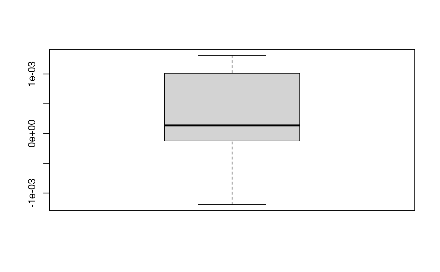 kfolds2Chisqind(bbb2)
#> [[1]]
#> [[1]][[1]]
#> [1] NA NA NA NA NA NA
#>
#> [[1]][[2]]
#> [1] NA NA NA NA NA NA
#>
#> [[1]][[3]]
#> [1] NA NA NA NA NA
#>
#> [[1]][[4]]
#> [1] NA NA NA NA NA NA
#>
#> [[1]][[5]]
#> [1] NA NA NA NA NA NA
#>
#>
kfolds2Chisq(bbb2)
#> [[1]]
#> [1] NA NA NA NA NA
#>
summary(bbb2)
#> ____************************************************____
#>
#> Family: inverse.gaussian
#> Link function: 1/mu^2
#>
#> ____Component____ 1 ____
#> ____Component____ 2 ____
#> ____Component____ 3 ____
#> ____Component____ 4 ____
#> ____Component____ 5 ____
#> ____Component____ 6 ____
#> ____Predicting X without NA neither in X or Y____
#> ****________________________________________________****
#>
#>
#> NK: 1
#> [[1]]
#> AIC BIC Q2Chisqcum_Y limQ2 Q2Chisq_Y PREChi2_Pearson_Y
#> Nb_Comp_0 81.67928 82.64909 NA NA NA NA
#> Nb_Comp_1 49.90521 51.35993 NA 0.0975 NA NA
#> Nb_Comp_2 31.06918 33.00881 NA 0.0975 NA NA
#> Nb_Comp_3 28.40632 30.83085 NA 0.0975 NA NA
#> Nb_Comp_4 27.08522 29.99466 NA 0.0975 NA NA
#> Nb_Comp_5 28.46056 31.85490 NA 0.0975 NA NA
#> Nb_Comp_6 29.68366 33.56292 NA 0.0975 NA NA
#> Chi2_Pearson_Y RSS_Y R2_Y
#> Nb_Comp_0 6.729783e-04 467.796667 NA
#> Nb_Comp_1 3.957680e-05 32.478677 0.9305710
#> Nb_Comp_2 7.009452e-06 6.020269 0.9871306
#> Nb_Comp_3 4.727777e-06 3.795855 0.9918857
#> Nb_Comp_4 3.584346e-06 2.699884 0.9942285
#> Nb_Comp_5 3.408069e-06 2.598572 0.9944451
#> Nb_Comp_6 3.195402e-06 2.492371 0.9946721
#>
#> attr(,"class")
#> [1] "summary.cv.plsRglmmodel"
PLS_lm_formula(Y~.,data=Cornell,10,typeVC="standard")$InfCrit
#> ____************************************************____
#> ____TypeVC____ standard ____
#> ____Component____ 1 ____
#> ____Component____ 2 ____
#> ____Component____ 3 ____
#> ____Component____ 4 ____
#> ____Component____ 5 ____
#> ____Component____ 6 ____
#> Warning : 1 2 3 4 5 6 7 < 10^{-12}
#> Warning only 6 components could thus be extracted
#> ____Predicting X without NA neither in X nor in Y____
#> ****________________________________________________****
#>
#> AIC Q2cum_Y LimQ2_Y Q2_Y PRESS_Y RSS_Y R2_Y
#> Nb_Comp_0 82.01205 NA NA NA NA 467.796667 NA
#> Nb_Comp_1 53.15173 0.8966556 0.0975 0.89665563 48.344150 35.742486 0.9235940
#> Nb_Comp_2 41.08283 0.9175426 0.0975 0.20210989 28.518576 11.066606 0.9763431
#> Nb_Comp_3 32.06411 0.9399676 0.0975 0.27195907 8.056942 4.418081 0.9905556
#> Nb_Comp_4 33.76477 0.9197009 0.0975 -0.33759604 5.909608 4.309235 0.9907882
#> Nb_Comp_5 33.34373 0.9281373 0.0975 0.10506161 3.856500 3.521924 0.9924713
#> Nb_Comp_6 35.25533 0.9232562 0.0975 -0.06792167 3.761138 3.496074 0.9925265
#> R2_residY RSS_residY PRESS_residY Q2_residY LimQ2 Q2cum_residY
#> Nb_Comp_0 NA 11.00000000 NA NA NA NA
#> Nb_Comp_1 0.9235940 0.84046633 1.13678803 0.89665563 0.0975 0.8966556
#> Nb_Comp_2 0.9763431 0.26022559 0.67059977 0.20210989 0.0975 0.9175426
#> Nb_Comp_3 0.9905556 0.10388893 0.18945488 0.27195907 0.0975 0.9399676
#> Nb_Comp_4 0.9907882 0.10132947 0.13896142 -0.33759604 0.0975 0.9197009
#> Nb_Comp_5 0.9924713 0.08281624 0.09068364 0.10506161 0.0975 0.9281373
#> Nb_Comp_6 0.9925265 0.08220840 0.08844125 -0.06792167 0.0975 0.9232562
#> AIC.std DoF.dof sigmahat.dof AIC.dof BIC.dof GMDL.dof
#> Nb_Comp_0 37.010388 1.000000 6.5212706 46.0708838 47.7893514 27.59461
#> Nb_Comp_1 8.150064 2.740749 1.8665281 4.5699686 4.9558156 21.34020
#> Nb_Comp_2 -3.918831 5.085967 1.1825195 2.1075461 2.3949331 27.40202
#> Nb_Comp_3 -12.937550 5.121086 0.7488308 0.8467795 0.9628191 24.40842
#> Nb_Comp_4 -11.236891 5.103312 0.7387162 0.8232505 0.9357846 24.23105
#> Nb_Comp_5 -11.657929 6.006316 0.7096382 0.7976101 0.9198348 28.21184
#> Nb_Comp_6 -9.746328 7.000001 0.7633342 0.9711319 1.1359499 33.18347
#> DoF.naive sigmahat.naive AIC.naive BIC.naive GMDL.naive
#> Nb_Comp_0 1 6.5212706 46.0708838 47.7893514 27.59461
#> Nb_Comp_1 2 1.8905683 4.1699567 4.4588195 18.37545
#> Nb_Comp_2 3 1.1088836 1.5370286 1.6860917 17.71117
#> Nb_Comp_3 4 0.7431421 0.7363469 0.8256118 19.01033
#> Nb_Comp_4 5 0.7846050 0.8721072 0.9964867 24.16510
#> Nb_Comp_5 6 0.7661509 0.8804809 1.0227979 28.64206
#> Nb_Comp_6 7 0.8361907 1.1070902 1.3048716 33.63927
rm(list=c("bbb","bbb2"))
#> Warning: object 'bbb' not found
data(bordeaux)
summary(cv.plsRglm(Quality~.,data=bordeaux,10,
modele="pls-glm-polr",K=7))
#>
#> Model: pls-glm-polr
#> Method: logistic
#>
#> NK: 1
#> Number of groups : 7
#> 1
#> ____************************************************____
#>
#> Model: pls-glm-polr
#> Method: logistic
#>
#> ____Predicting X without NA neither in X nor in Y____
#> ____Component____ 1 ____
#> ____Component____ 2 ____
#> ____Component____ 3 ____
#> ____Component____ 4 ____
#> Warning : < 10^{-12}
#> Warning only 4 components could thus be extracted
#> ****________________________________________________****
#>
#> 2
#> ____************************************************____
#>
#> Model: pls-glm-polr
#> Method: logistic
#>
#> ____Predicting X without NA neither in X nor in Y____
#> ____Component____ 1 ____
#> ____Component____ 2 ____
#> ____Component____ 3 ____
#> Warning: glm.fit: fitted probabilities numerically 0 or 1 occurred
#> Warning: glm.fit: fitted probabilities numerically 0 or 1 occurred
#> Warning: glm.fit: fitted probabilities numerically 0 or 1 occurred
#> Warning: glm.fit: fitted probabilities numerically 0 or 1 occurred
#> Warning: glm.fit: fitted probabilities numerically 0 or 1 occurred
#> ____Component____ 4 ____
#> Warning : < 10^{-12}
#> Warning only 4 components could thus be extracted
#> ****________________________________________________****
#>
#> 3
#> ____************************************************____
#>
#> Model: pls-glm-polr
#> Method: logistic
#>
#> ____Predicting X without NA neither in X nor in Y____
#> ____Component____ 1 ____
#> ____Component____ 2 ____
#> ____Component____ 3 ____
#> ____Component____ 4 ____
#> Warning : < 10^{-12}
#> Warning only 4 components could thus be extracted
#> ****________________________________________________****
#>
#> 4
#> ____************************************************____
#>
#> Model: pls-glm-polr
#> Method: logistic
#>
#> ____Predicting X without NA neither in X nor in Y____
#> ____Component____ 1 ____
#> ____Component____ 2 ____
#> ____Component____ 3 ____
#> ____Component____ 4 ____
#> Warning : < 10^{-12}
#> Warning only 4 components could thus be extracted
#> ****________________________________________________****
#>
#> 5
#> ____************************************************____
#>
#> Model: pls-glm-polr
#> Method: logistic
#>
#> ____Predicting X without NA neither in X nor in Y____
#> ____Component____ 1 ____
#> ____Component____ 2 ____
#> ____Component____ 3 ____
#> ____Component____ 4 ____
#> Warning : < 10^{-12}
#> Warning only 4 components could thus be extracted
#> ****________________________________________________****
#>
#> 6
#> ____************************************************____
#>
#> Model: pls-glm-polr
#> Method: logistic
#>
#> ____Predicting X without NA neither in X nor in Y____
#> ____Component____ 1 ____
#> ____Component____ 2 ____
#> ____Component____ 3 ____
#> ____Component____ 4 ____
#> Warning : < 10^{-12}
#> Warning only 4 components could thus be extracted
#> ****________________________________________________****
#>
#> 7
#> ____************************************************____
#>
#> Model: pls-glm-polr
#> Method: logistic
#>
#> ____Predicting X without NA neither in X nor in Y____
#> ____Component____ 1 ____
#> ____Component____ 2 ____
#> ____Component____ 3 ____
#> ____Component____ 4 ____
#> Warning : < 10^{-12}
#> Warning only 4 components could thus be extracted
#> ****________________________________________________****
#>
#> ____************************************************____
#>
#> Model: pls-glm-polr
#> Method: logistic
#>
#> ____Component____ 1 ____
#> ____Predicting X without NA neither in X or Y____
#> ****________________________________________________****
#>
#>
#> NK: 1
#> [[1]]
#> AIC BIC Q2Chisqcum_Y limQ2 Q2Chisq_Y PREChi2_Pearson_Y
#> Nb_Comp_0 78.64736 81.70009 NA NA NA NA
#> Nb_Comp_1 36.50286 41.08194 -0.2712984 0.0975 -0.2712984 79.24427
#> Chi2_Pearson_Y
#> Nb_Comp_0 62.333333
#> Nb_Comp_1 9.356521
#>
#> attr(,"class")
#> [1] "summary.cv.plsRglmmodel"
data(bordeauxNA)
summary(cv.plsRglm(Quality~.,data=bordeauxNA,
10,modele="pls-glm-polr",K=10,verbose=FALSE))
#> ____************************************************____
#> Only naive DoF can be used with missing data
#>
#> Model: pls-glm-polr
#> Method: logistic
#>
#> ____There are some NAs in X but not in Y____
#> ____Component____ 1 ____
#> ____Predicting X with NA in X and not in Y____
#> ****________________________________________________****
#>
#>
#> NK: 1
#> [[1]]
#> AIC BIC Q2Chisqcum_Y limQ2 Q2Chisq_Y PREChi2_Pearson_Y
#> Nb_Comp_0 78.64736 81.70009 NA NA NA NA
#> Nb_Comp_1 36.21263 40.79171 -0.952643 0.0975 -0.952643 121.7147
#> Chi2_Pearson_Y
#> Nb_Comp_0 62.333333
#> Nb_Comp_1 9.454055
#>
#> attr(,"class")
#> [1] "summary.cv.plsRglmmodel"
summary(cv.plsRglm(Quality~.,data=bordeaux,nt=2,K=7,
modele="pls-glm-polr",method="logistic",verbose=FALSE))
#> Warning: glm.fit: fitted probabilities numerically 0 or 1 occurred
#> Warning: glm.fit: algorithm did not converge
#> Warning: glm.fit: fitted probabilities numerically 0 or 1 occurred
#> ____************************************************____
#>
#> Model: pls-glm-polr
#> Method: logistic
#>
#> ____Component____ 1 ____
#> ____Predicting X without NA neither in X or Y____
#> ****________________________________________________****
#>
#>
#> NK: 1
#> [[1]]
#> AIC BIC Q2Chisqcum_Y limQ2 Q2Chisq_Y PREChi2_Pearson_Y
#> Nb_Comp_0 78.64736 81.70009 NA NA NA NA
#> Nb_Comp_1 36.50286 41.08194 -0.398239 0.0975 -0.398239 87.1569
#> Chi2_Pearson_Y
#> Nb_Comp_0 62.333333
#> Nb_Comp_1 9.356521
#>
#> attr(,"class")
#> [1] "summary.cv.plsRglmmodel"
summary(cv.plsRglm(Quality~.,data=bordeaux,nt=2,K=7,
modele="pls-glm-polr",method="probit",verbose=FALSE))
#> Warning: glm.fit: fitted probabilities numerically 0 or 1 occurred
#> Warning: glm.fit: fitted probabilities numerically 0 or 1 occurred
#> ____************************************************____
#>
#> Model: pls-glm-polr
#> Method: probit
#>
#> ____Component____ 1 ____
#> ____Predicting X without NA neither in X or Y____
#> ****________________________________________________****
#>
#>
#> NK: 1
#> [[1]]
#> AIC BIC Q2Chisqcum_Y limQ2 Q2Chisq_Y PREChi2_Pearson_Y
#> Nb_Comp_0 78.64736 81.70009 NA NA NA NA
#> Nb_Comp_1 36.01661 40.59569 -1.784808 0.0975 -1.784808 173.5868
#> Chi2_Pearson_Y
#> Nb_Comp_0 62.33350
#> Nb_Comp_1 9.71675
#>
#> attr(,"class")
#> [1] "summary.cv.plsRglmmodel"
summary(cv.plsRglm(Quality~.,data=bordeaux,nt=2,K=7,
modele="pls-glm-polr",method="cloglog",verbose=FALSE))
#> ____************************************************____
#>
#> Model: pls-glm-polr
#> Method: cloglog
#>
#> ____Component____ 1 ____
#> ____Predicting X without NA neither in X or Y____
#> ****________________________________________________****
#>
#>
#> NK: 1
#> [[1]]
#> AIC BIC Q2Chisqcum_Y limQ2 Q2Chisq_Y PREChi2_Pearson_Y
#> Nb_Comp_0 78.64736 81.70009 NA NA NA NA
#> Nb_Comp_1 36.92722 41.50630 -1590108 0.0975 -1590108 99119030
#> Chi2_Pearson_Y
#> Nb_Comp_0 62.33474
#> Nb_Comp_1 10.32213
#>
#> attr(,"class")
#> [1] "summary.cv.plsRglmmodel"
suppressWarnings(summary(cv.plsRglm(Quality~.,data=bordeaux,nt=2,K=7,
modele="pls-glm-polr",method="cauchit",verbose=FALSE)))
#> ____************************************************____
#>
#> Model: pls-glm-polr
#> Method: cauchit
#>
#> ____Component____ 1 ____
#> ____Predicting X without NA neither in X or Y____
#> ****________________________________________________****
#>
#>
#> NK: 1
#> [[1]]
#> AIC BIC Q2Chisqcum_Y limQ2 Q2Chisq_Y PREChi2_Pearson_Y
#> Nb_Comp_0 79.08163 82.13436 NA NA NA NA
#> Nb_Comp_1 38.11253 42.69161 -0.2568805 0.0975 -0.2568805 78.02523
#> Chi2_Pearson_Y
#> Nb_Comp_0 62.078483
#> Nb_Comp_1 8.592708
#>
#> attr(,"class")
#> [1] "summary.cv.plsRglmmodel"
# }
kfolds2Chisqind(bbb2)
#> [[1]]
#> [[1]][[1]]
#> [1] NA NA NA NA NA NA
#>
#> [[1]][[2]]
#> [1] NA NA NA NA NA NA
#>
#> [[1]][[3]]
#> [1] NA NA NA NA NA
#>
#> [[1]][[4]]
#> [1] NA NA NA NA NA NA
#>
#> [[1]][[5]]
#> [1] NA NA NA NA NA NA
#>
#>
kfolds2Chisq(bbb2)
#> [[1]]
#> [1] NA NA NA NA NA
#>
summary(bbb2)
#> ____************************************************____
#>
#> Family: inverse.gaussian
#> Link function: 1/mu^2
#>
#> ____Component____ 1 ____
#> ____Component____ 2 ____
#> ____Component____ 3 ____
#> ____Component____ 4 ____
#> ____Component____ 5 ____
#> ____Component____ 6 ____
#> ____Predicting X without NA neither in X or Y____
#> ****________________________________________________****
#>
#>
#> NK: 1
#> [[1]]
#> AIC BIC Q2Chisqcum_Y limQ2 Q2Chisq_Y PREChi2_Pearson_Y
#> Nb_Comp_0 81.67928 82.64909 NA NA NA NA
#> Nb_Comp_1 49.90521 51.35993 NA 0.0975 NA NA
#> Nb_Comp_2 31.06918 33.00881 NA 0.0975 NA NA
#> Nb_Comp_3 28.40632 30.83085 NA 0.0975 NA NA
#> Nb_Comp_4 27.08522 29.99466 NA 0.0975 NA NA
#> Nb_Comp_5 28.46056 31.85490 NA 0.0975 NA NA
#> Nb_Comp_6 29.68366 33.56292 NA 0.0975 NA NA
#> Chi2_Pearson_Y RSS_Y R2_Y
#> Nb_Comp_0 6.729783e-04 467.796667 NA
#> Nb_Comp_1 3.957680e-05 32.478677 0.9305710
#> Nb_Comp_2 7.009452e-06 6.020269 0.9871306
#> Nb_Comp_3 4.727777e-06 3.795855 0.9918857
#> Nb_Comp_4 3.584346e-06 2.699884 0.9942285
#> Nb_Comp_5 3.408069e-06 2.598572 0.9944451
#> Nb_Comp_6 3.195402e-06 2.492371 0.9946721
#>
#> attr(,"class")
#> [1] "summary.cv.plsRglmmodel"
PLS_lm_formula(Y~.,data=Cornell,10,typeVC="standard")$InfCrit
#> ____************************************************____
#> ____TypeVC____ standard ____
#> ____Component____ 1 ____
#> ____Component____ 2 ____
#> ____Component____ 3 ____
#> ____Component____ 4 ____
#> ____Component____ 5 ____
#> ____Component____ 6 ____
#> Warning : 1 2 3 4 5 6 7 < 10^{-12}
#> Warning only 6 components could thus be extracted
#> ____Predicting X without NA neither in X nor in Y____
#> ****________________________________________________****
#>
#> AIC Q2cum_Y LimQ2_Y Q2_Y PRESS_Y RSS_Y R2_Y
#> Nb_Comp_0 82.01205 NA NA NA NA 467.796667 NA
#> Nb_Comp_1 53.15173 0.8966556 0.0975 0.89665563 48.344150 35.742486 0.9235940
#> Nb_Comp_2 41.08283 0.9175426 0.0975 0.20210989 28.518576 11.066606 0.9763431
#> Nb_Comp_3 32.06411 0.9399676 0.0975 0.27195907 8.056942 4.418081 0.9905556
#> Nb_Comp_4 33.76477 0.9197009 0.0975 -0.33759604 5.909608 4.309235 0.9907882
#> Nb_Comp_5 33.34373 0.9281373 0.0975 0.10506161 3.856500 3.521924 0.9924713
#> Nb_Comp_6 35.25533 0.9232562 0.0975 -0.06792167 3.761138 3.496074 0.9925265
#> R2_residY RSS_residY PRESS_residY Q2_residY LimQ2 Q2cum_residY
#> Nb_Comp_0 NA 11.00000000 NA NA NA NA
#> Nb_Comp_1 0.9235940 0.84046633 1.13678803 0.89665563 0.0975 0.8966556
#> Nb_Comp_2 0.9763431 0.26022559 0.67059977 0.20210989 0.0975 0.9175426
#> Nb_Comp_3 0.9905556 0.10388893 0.18945488 0.27195907 0.0975 0.9399676
#> Nb_Comp_4 0.9907882 0.10132947 0.13896142 -0.33759604 0.0975 0.9197009
#> Nb_Comp_5 0.9924713 0.08281624 0.09068364 0.10506161 0.0975 0.9281373
#> Nb_Comp_6 0.9925265 0.08220840 0.08844125 -0.06792167 0.0975 0.9232562
#> AIC.std DoF.dof sigmahat.dof AIC.dof BIC.dof GMDL.dof
#> Nb_Comp_0 37.010388 1.000000 6.5212706 46.0708838 47.7893514 27.59461
#> Nb_Comp_1 8.150064 2.740749 1.8665281 4.5699686 4.9558156 21.34020
#> Nb_Comp_2 -3.918831 5.085967 1.1825195 2.1075461 2.3949331 27.40202
#> Nb_Comp_3 -12.937550 5.121086 0.7488308 0.8467795 0.9628191 24.40842
#> Nb_Comp_4 -11.236891 5.103312 0.7387162 0.8232505 0.9357846 24.23105
#> Nb_Comp_5 -11.657929 6.006316 0.7096382 0.7976101 0.9198348 28.21184
#> Nb_Comp_6 -9.746328 7.000001 0.7633342 0.9711319 1.1359499 33.18347
#> DoF.naive sigmahat.naive AIC.naive BIC.naive GMDL.naive
#> Nb_Comp_0 1 6.5212706 46.0708838 47.7893514 27.59461
#> Nb_Comp_1 2 1.8905683 4.1699567 4.4588195 18.37545
#> Nb_Comp_2 3 1.1088836 1.5370286 1.6860917 17.71117
#> Nb_Comp_3 4 0.7431421 0.7363469 0.8256118 19.01033
#> Nb_Comp_4 5 0.7846050 0.8721072 0.9964867 24.16510
#> Nb_Comp_5 6 0.7661509 0.8804809 1.0227979 28.64206
#> Nb_Comp_6 7 0.8361907 1.1070902 1.3048716 33.63927
rm(list=c("bbb","bbb2"))
#> Warning: object 'bbb' not found
data(bordeaux)
summary(cv.plsRglm(Quality~.,data=bordeaux,10,
modele="pls-glm-polr",K=7))
#>
#> Model: pls-glm-polr
#> Method: logistic
#>
#> NK: 1
#> Number of groups : 7
#> 1
#> ____************************************************____
#>
#> Model: pls-glm-polr
#> Method: logistic
#>
#> ____Predicting X without NA neither in X nor in Y____
#> ____Component____ 1 ____
#> ____Component____ 2 ____
#> ____Component____ 3 ____
#> ____Component____ 4 ____
#> Warning : < 10^{-12}
#> Warning only 4 components could thus be extracted
#> ****________________________________________________****
#>
#> 2
#> ____************************************************____
#>
#> Model: pls-glm-polr
#> Method: logistic
#>
#> ____Predicting X without NA neither in X nor in Y____
#> ____Component____ 1 ____
#> ____Component____ 2 ____
#> ____Component____ 3 ____
#> Warning: glm.fit: fitted probabilities numerically 0 or 1 occurred
#> Warning: glm.fit: fitted probabilities numerically 0 or 1 occurred
#> Warning: glm.fit: fitted probabilities numerically 0 or 1 occurred
#> Warning: glm.fit: fitted probabilities numerically 0 or 1 occurred
#> Warning: glm.fit: fitted probabilities numerically 0 or 1 occurred
#> ____Component____ 4 ____
#> Warning : < 10^{-12}
#> Warning only 4 components could thus be extracted
#> ****________________________________________________****
#>
#> 3
#> ____************************************************____
#>
#> Model: pls-glm-polr
#> Method: logistic
#>
#> ____Predicting X without NA neither in X nor in Y____
#> ____Component____ 1 ____
#> ____Component____ 2 ____
#> ____Component____ 3 ____
#> ____Component____ 4 ____
#> Warning : < 10^{-12}
#> Warning only 4 components could thus be extracted
#> ****________________________________________________****
#>
#> 4
#> ____************************************************____
#>
#> Model: pls-glm-polr
#> Method: logistic
#>
#> ____Predicting X without NA neither in X nor in Y____
#> ____Component____ 1 ____
#> ____Component____ 2 ____
#> ____Component____ 3 ____
#> ____Component____ 4 ____
#> Warning : < 10^{-12}
#> Warning only 4 components could thus be extracted
#> ****________________________________________________****
#>
#> 5
#> ____************************************************____
#>
#> Model: pls-glm-polr
#> Method: logistic
#>
#> ____Predicting X without NA neither in X nor in Y____
#> ____Component____ 1 ____
#> ____Component____ 2 ____
#> ____Component____ 3 ____
#> ____Component____ 4 ____
#> Warning : < 10^{-12}
#> Warning only 4 components could thus be extracted
#> ****________________________________________________****
#>
#> 6
#> ____************************************************____
#>
#> Model: pls-glm-polr
#> Method: logistic
#>
#> ____Predicting X without NA neither in X nor in Y____
#> ____Component____ 1 ____
#> ____Component____ 2 ____
#> ____Component____ 3 ____
#> ____Component____ 4 ____
#> Warning : < 10^{-12}
#> Warning only 4 components could thus be extracted
#> ****________________________________________________****
#>
#> 7
#> ____************************************************____
#>
#> Model: pls-glm-polr
#> Method: logistic
#>
#> ____Predicting X without NA neither in X nor in Y____
#> ____Component____ 1 ____
#> ____Component____ 2 ____
#> ____Component____ 3 ____
#> ____Component____ 4 ____
#> Warning : < 10^{-12}
#> Warning only 4 components could thus be extracted
#> ****________________________________________________****
#>
#> ____************************************************____
#>
#> Model: pls-glm-polr
#> Method: logistic
#>
#> ____Component____ 1 ____
#> ____Predicting X without NA neither in X or Y____
#> ****________________________________________________****
#>
#>
#> NK: 1
#> [[1]]
#> AIC BIC Q2Chisqcum_Y limQ2 Q2Chisq_Y PREChi2_Pearson_Y
#> Nb_Comp_0 78.64736 81.70009 NA NA NA NA
#> Nb_Comp_1 36.50286 41.08194 -0.2712984 0.0975 -0.2712984 79.24427
#> Chi2_Pearson_Y
#> Nb_Comp_0 62.333333
#> Nb_Comp_1 9.356521
#>
#> attr(,"class")
#> [1] "summary.cv.plsRglmmodel"
data(bordeauxNA)
summary(cv.plsRglm(Quality~.,data=bordeauxNA,
10,modele="pls-glm-polr",K=10,verbose=FALSE))
#> ____************************************************____
#> Only naive DoF can be used with missing data
#>
#> Model: pls-glm-polr
#> Method: logistic
#>
#> ____There are some NAs in X but not in Y____
#> ____Component____ 1 ____
#> ____Predicting X with NA in X and not in Y____
#> ****________________________________________________****
#>
#>
#> NK: 1
#> [[1]]
#> AIC BIC Q2Chisqcum_Y limQ2 Q2Chisq_Y PREChi2_Pearson_Y
#> Nb_Comp_0 78.64736 81.70009 NA NA NA NA
#> Nb_Comp_1 36.21263 40.79171 -0.952643 0.0975 -0.952643 121.7147
#> Chi2_Pearson_Y
#> Nb_Comp_0 62.333333
#> Nb_Comp_1 9.454055
#>
#> attr(,"class")
#> [1] "summary.cv.plsRglmmodel"
summary(cv.plsRglm(Quality~.,data=bordeaux,nt=2,K=7,
modele="pls-glm-polr",method="logistic",verbose=FALSE))
#> Warning: glm.fit: fitted probabilities numerically 0 or 1 occurred
#> Warning: glm.fit: algorithm did not converge
#> Warning: glm.fit: fitted probabilities numerically 0 or 1 occurred
#> ____************************************************____
#>
#> Model: pls-glm-polr
#> Method: logistic
#>
#> ____Component____ 1 ____
#> ____Predicting X without NA neither in X or Y____
#> ****________________________________________________****
#>
#>
#> NK: 1
#> [[1]]
#> AIC BIC Q2Chisqcum_Y limQ2 Q2Chisq_Y PREChi2_Pearson_Y
#> Nb_Comp_0 78.64736 81.70009 NA NA NA NA
#> Nb_Comp_1 36.50286 41.08194 -0.398239 0.0975 -0.398239 87.1569
#> Chi2_Pearson_Y
#> Nb_Comp_0 62.333333
#> Nb_Comp_1 9.356521
#>
#> attr(,"class")
#> [1] "summary.cv.plsRglmmodel"
summary(cv.plsRglm(Quality~.,data=bordeaux,nt=2,K=7,
modele="pls-glm-polr",method="probit",verbose=FALSE))
#> Warning: glm.fit: fitted probabilities numerically 0 or 1 occurred
#> Warning: glm.fit: fitted probabilities numerically 0 or 1 occurred
#> ____************************************************____
#>
#> Model: pls-glm-polr
#> Method: probit
#>
#> ____Component____ 1 ____
#> ____Predicting X without NA neither in X or Y____
#> ****________________________________________________****
#>
#>
#> NK: 1
#> [[1]]
#> AIC BIC Q2Chisqcum_Y limQ2 Q2Chisq_Y PREChi2_Pearson_Y
#> Nb_Comp_0 78.64736 81.70009 NA NA NA NA
#> Nb_Comp_1 36.01661 40.59569 -1.784808 0.0975 -1.784808 173.5868
#> Chi2_Pearson_Y
#> Nb_Comp_0 62.33350
#> Nb_Comp_1 9.71675
#>
#> attr(,"class")
#> [1] "summary.cv.plsRglmmodel"
summary(cv.plsRglm(Quality~.,data=bordeaux,nt=2,K=7,
modele="pls-glm-polr",method="cloglog",verbose=FALSE))
#> ____************************************************____
#>
#> Model: pls-glm-polr
#> Method: cloglog
#>
#> ____Component____ 1 ____
#> ____Predicting X without NA neither in X or Y____
#> ****________________________________________________****
#>
#>
#> NK: 1
#> [[1]]
#> AIC BIC Q2Chisqcum_Y limQ2 Q2Chisq_Y PREChi2_Pearson_Y
#> Nb_Comp_0 78.64736 81.70009 NA NA NA NA
#> Nb_Comp_1 36.92722 41.50630 -1590108 0.0975 -1590108 99119030
#> Chi2_Pearson_Y
#> Nb_Comp_0 62.33474
#> Nb_Comp_1 10.32213
#>
#> attr(,"class")
#> [1] "summary.cv.plsRglmmodel"
suppressWarnings(summary(cv.plsRglm(Quality~.,data=bordeaux,nt=2,K=7,
modele="pls-glm-polr",method="cauchit",verbose=FALSE)))
#> ____************************************************____
#>
#> Model: pls-glm-polr
#> Method: cauchit
#>
#> ____Component____ 1 ____
#> ____Predicting X without NA neither in X or Y____
#> ****________________________________________________****
#>
#>
#> NK: 1
#> [[1]]
#> AIC BIC Q2Chisqcum_Y limQ2 Q2Chisq_Y PREChi2_Pearson_Y
#> Nb_Comp_0 79.08163 82.13436 NA NA NA NA
#> Nb_Comp_1 38.11253 42.69161 -0.2568805 0.0975 -0.2568805 78.02523
#> Chi2_Pearson_Y
#> Nb_Comp_0 62.078483
#> Nb_Comp_1 8.592708
#>
#> attr(,"class")
#> [1] "summary.cv.plsRglmmodel"
# }