Chapitre 02. Statistiques descriptives et visualisation des données univariables.
Tout le code avec R.
F. Bertrand et M. Maumy
2025-09-22
Source:vignettes/CodeChap02.Rmd
CodeChap02.Rmd

|
|
Sources des données
Statistique Canada
Données libres d’utilisation, commerciale ou non, sur Statistique Canada. https://www.statcan.gc.ca/fra/reference/droit-auteur
répartition en classes d’âge de la population du Canada en 2020. Statistique Canada. Tableau 17-10-0005-01 Estimations de la population au 1er juillet, par âge et sexe DOI : https://doi.org/10.25318/1710000501-fra
population des dix provinces et trois territoires du Canada au quatrième trimestre 2020. Source : Statistique Canada. Tableau 17-10-0009-01. Estimations de la population, trimestrielles. DOI : https://doi.org/10.25318/1710000901-fra
Statistique de l’OCDE.
- Taux d’emploi en % de la classe d’age
Taux d’emploi par groupe d’âge (indicateur). OCDE (2021). doi: 10.1787/b01db125-fr (Consulté le 11 février 2021)
Le taux d’emploi d’une classe d’âge se mesure en fonction du nombre des actifs occupés d’un âge donné rapporté à l’effectif total de cette classe d’âge. Les actifs occupés sont les personnes de 15 ans et plus qui, durant la semaine de référence, déclarent avoir effectué un travail rémunéré pendant une heure au moins ou avoir occupé un emploi dont elles étaient absentes. Les taux d’emploi sont présentés pour quatre classes d’âge : les personnes âgées de 15 à 64 ans (personnes en âge de travailler); les personnes âgées de 15 à 24 ans sont celles qui font leur entrée sur le marché du travail à l’issue de leur scolarité, les personnes âgées de 25 à 54 ans sont celles qui sont au plus fort de leur activité professionnelle, et les personnes âgées de 55 à 64 ans sont celles qui ont dépassé le pic de leur carrière professionnelle et approchent de l’âge de la retraite. Cet indicateur est désaisonnalisé et est mesuré en pourcentage de l’effectif total de la classe d’âge.
- Par secteur dans les pays de l’OCDE en 2020-Q3.
Emploi par activité (indicateur). OCDE (2021). doi: 10.1787/6b2fff89-fr (Consulté le 11 février 2021)
- Emploi par niveau d’études en % des 25-64 ans
Emploi par niveau d’études (indicateur). OCDE (2021) doi: 10.1787/6e3d44f3-fr (Consulté le 11 février 2021)
Cet indicateur fournit les taux d’emploi selon le niveau d’études : premier cycle du second degré, deuxième cycle du second degré, supérieur. Le taux d’emploi est le pourcentage d’actifs occupés dans la population en âge de travailler. Les actifs occupés sont les personnes qui travaillent au moins une heure par semaine en tant que salarié ou à titre lucratif, ou qui ont un emploi mais sont temporairement absentes de leur travail pour maladie, congé ou conflit social. Cet indicateur donne le pourcentage des actifs occupés âgés de 25 à 64 ans dans la population des individus âgés de 25 à 64 ans.
- Part du revenu national total équivalent en Euro en 2019. Répartitition du revenu par quantiles - enquêtes EU-SILC et PCM (ILC_DI01).
INSEE
- Ménages par taille du ménage,
MEN4 - Ménages par taille du ménage, sexe et âge de la personne de référence en 2017. France métropolitaine. Insee.
Données Covid officielles
Répartition par région française du nombre de personnes hospitalisées et atteintes du Covid 19 le 21 février 2021.
Répartition par région française du nombre de personne en réanimation et atteintes du Covid 19 le 21 février 2021.
if(!("sageR" %in% installed.packages())){install.packages("sageR")}
library(sageR)
Effectifs
Nombre de personnes dans un foyer Tableau 2.5
data(Personnes_Foyer)
xi <- Personnes_Foyer$xi
ni <- Personnes_Foyer$niDispersion
sqrt(weighted.mean((xi-weighted.mean(xi,ni))^2,ni))
#> [1] 1.246994
sqrt(weighted.mean((xi-weighted.mean(xi,ni))^2,ni))/weighted.mean(xi,ni)*100
#> [1] 56.89321

rrr=rep(xi, ni)
mean(rrr)
#> [1] 2.191815
quantile(rrr)
#>   0%  25%  50%  75% 100%
#>    1    1    2    3    6
median(abs(rrr-median(rrr)))
#> [1] 1
mad(rrr,constant = 1)
#> [1] 1
Population classes d’age Canada
data(AgevsProter_Canada_full)
Age <- margin.table(as.matrix(AgevsProter_Canada_full),1)
Age
#>       0 à 4 ans       5 à 9 ans     10 à 14 ans     15 à 19 ans     20 à 24 ans
#>         1921944         2044603         2072100         2100865         2482802
#>     25 à 29 ans     30 à 34 ans     35 à 39 ans     40 à 44 ans     45 à 49 ans
#>         2645240         2661723         2630680         2464247         2390116
#>     50 à 54 ans     55 à 59 ans     60 à 64 ans     65 à 69 ans     70 à 74 ans
#>         2449915         2744896         2560241         2167275         1786622
#>     75 à 79 ans     80 à 84 ans     85 à 89 ans     90 à 94 ans     95 à 99 ans
#>         1218303          811370          517710          248593           74476
#> 100 ans et plus
#>           11517
cumsum(Age)
#>       0 à 4 ans       5 à 9 ans     10 à 14 ans     15 à 19 ans     20 à 24 ans
#>         1921944         3966547         6038647         8139512        10622314
#>     25 à 29 ans     30 à 34 ans     35 à 39 ans     40 à 44 ans     45 à 49 ans
#>        13267554        15929277        18559957        21024204        23414320
#>     50 à 54 ans     55 à 59 ans     60 à 64 ans     65 à 69 ans     70 à 74 ans
#>        25864235        28609131        31169372        33336647        35123269
#>     75 à 79 ans     80 à 84 ans     85 à 89 ans     90 à 94 ans     95 à 99 ans
#>        36341572        37152942        37670652        37919245        37993721
#> 100 ans et plus
#>        38005238
Age/sum(Age)
#>       0 à 4 ans       5 à 9 ans     10 à 14 ans     15 à 19 ans     20 à 24 ans
#>    0.0505705029    0.0537979265    0.0545214320    0.0552783014    0.0653278898
#>     25 à 29 ans     30 à 34 ans     35 à 39 ans     40 à 44 ans     45 à 49 ans
#>    0.0696019849    0.0700356882    0.0692188798    0.0648396676    0.0628891207
#>     50 à 54 ans     55 à 59 ans     60 à 64 ans     65 à 69 ans     70 à 74 ans
#>    0.0644625617    0.0722241497    0.0673654774    0.0570256921    0.0470098885
#>     75 à 79 ans     80 à 84 ans     85 à 89 ans     90 à 94 ans     95 à 99 ans
#>    0.0320561866    0.0213488993    0.0136220697    0.0065410194    0.0019596246
#> 100 ans et plus
#>    0.0003030372
cumsum(Age)/sum(Age)
#>       0 à 4 ans       5 à 9 ans     10 à 14 ans     15 à 19 ans     20 à 24 ans
#>       0.0505705       0.1043684       0.1588899       0.2141682       0.2794961
#>     25 à 29 ans     30 à 34 ans     35 à 39 ans     40 à 44 ans     45 à 49 ans
#>       0.3490980       0.4191337       0.4883526       0.5531923       0.6160814
#>     50 à 54 ans     55 à 59 ans     60 à 64 ans     65 à 69 ans     70 à 74 ans
#>       0.6805440       0.7527681       0.8201336       0.8771593       0.9241692
#>     75 à 79 ans     80 à 84 ans     85 à 89 ans     90 à 94 ans     95 à 99 ans
#>       0.9562253       0.9775742       0.9911963       0.9977373       0.9996970
#> 100 ans et plus
#>       1.0000000
njall <- Age
nj <- njall[-length(njall)]
centres <- c(5*(0:19)+2.5)
cj <- 5*(0:20)
x <- actuar::grouped.data(Group = cj, Frequency = as.numeric(nj))
class(x)
#> [1] "grouped.data" "data.frame"Position
mean(x)
#> Frequency
#>  41.42872
quantile(x)
#>        0%       25%       50%       75%      100%
#>   0.00000  22.73666  40.88648  59.79263 100.00000
sum(nj*centres)/sum(nj)
#> [1] 41.42872

print(cumsum(nj/sum(nj)),digits=3)
#>   0 à 4 ans   5 à 9 ans 10 à 14 ans 15 à 19 ans 20 à 24 ans 25 à 29 ans
#>      0.0506      0.1044      0.1589      0.2142      0.2796      0.3492
#> 30 à 34 ans 35 à 39 ans 40 à 44 ans 45 à 49 ans 50 à 54 ans 55 à 59 ans
#>      0.4193      0.4885      0.5534      0.6163      0.6808      0.7530
#> 60 à 64 ans 65 à 69 ans 70 à 74 ans 75 à 79 ans 80 à 84 ans 85 à 89 ans
#>      0.8204      0.8774      0.9244      0.9565      0.9779      0.9915
#> 90 à 94 ans 95 à 99 ans
#>      0.9980      1.0000
centres
#>  [1]  2.5  7.5 12.5 17.5 22.5 27.5 32.5 37.5 42.5 47.5 52.5 57.5 62.5 67.5 72.5
#> [16] 77.5 82.5 87.5 92.5 97.5

40+(45-40)*(.5-0.4885)/(0.5534-0.4885)
#> [1] 40.88598
40.88598
#> [1] 40.88598

20+(25-20)*(0.2500-0.2142)/(0.2796-0.2142)
#> [1] 22.737
22.74
#> [1] 22.74

55 + (60-55)*(0.75-0.6808)/(0.7530-0.6808)
#> [1] 59.79224
59.79224
#> [1] 59.79224
Dispersion
59.79-22.74
#> [1] 37.05

#Centres
(x[,1][-1]+x[,1][-length(x[,1])])/2
#>  [1]  2.5  7.5 12.5 17.5 22.5 27.5 32.5 37.5 42.5 47.5 52.5 57.5 62.5 67.5 72.5
#> [16] 77.5 82.5 87.5 92.5 97.5

#sd
sqrt(weighted.mean(((x[,1][-1]+x[,1][-length(x[,1])])/2-mean(x))^2,x[,2])-1/12*weighted.mean(diff(x[,1])^2,x[,2]))
#> [1] 23.02927

#CV%
sqrt(weighted.mean(((x[,1][-1]+x[,1][-length(x[,1])])/2-mean(x))^2,x[,2])-1/12*weighted.mean(diff(x[,1])^2,x[,2]))/mean(x)*100
#> Frequency
#>  55.58769
Concentration
Lorentz
if(!("ggplot2" %in% installed.packages())){install.packages("ggplot2")}
library(ggplot2)
if(!("gglorenz" %in% installed.packages())){install.packages("gglorenz")}
library(gglorenz)
Jeu de données d’exemple du package gglorenz
ggplot(billionaires, aes(TNW)) +
    stat_lorenz()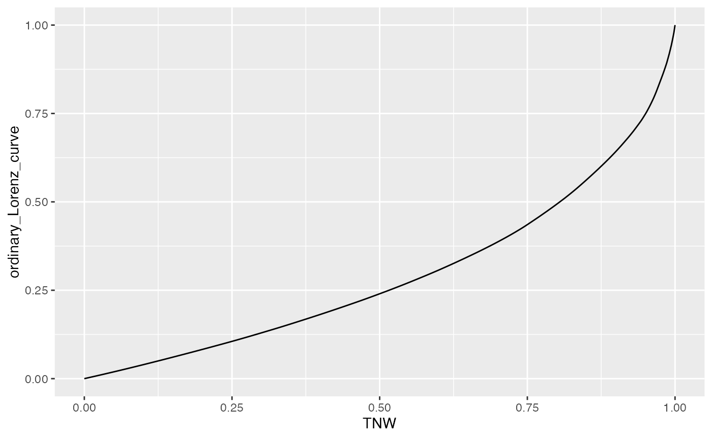
ggplot(billionaires, aes(TNW)) +
    stat_lorenz(desc = TRUE) +
    coord_fixed() +
    geom_abline(linetype = "dashed") +
    theme_minimal()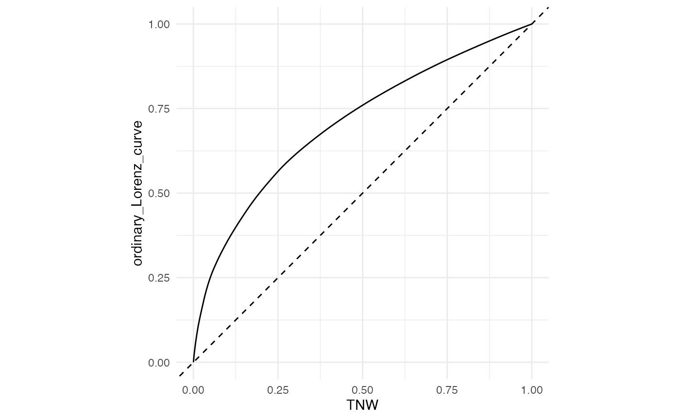
Répartition de la richesse dans les pays de l’OCDE
data(Richesse)
if(!("ggplot2" %in% installed.packages())){install.packages("ggplot2")}
library(ggplot2)
ggplot(Richesse, aes(Belgique)) +
    stat_lorenz() +
    coord_fixed() +
    geom_abline(linetype = "dashed") +
    theme_minimal() +
  ylab("Courbe de Lorenz ordinaire") +
  annotate_ineq(Richesse$Belgique,
  measure_ineq = "Gini")
Chemin = "~/Documents/Recherche/DeBoeck/Graphes/Donnees/"
colmodel="cmyk"
ggsave(filename = paste(Chemin,"Lorenz_Belgique.pdf",sep=""),
       width = 8, height = 7, onefile = TRUE, family = "Helvetica",
    title = "Lorenz curve", paper = "special", colormodel = colmodel)
ggplot(Richesse, aes(France)) +
    stat_lorenz() +
    coord_fixed() +
    geom_abline(linetype = "dashed") +
    theme_minimal() +
  ylab("Courbe de Lorenz ordinaire") +
  annotate_ineq(Richesse$France,
  measure_ineq = "Gini")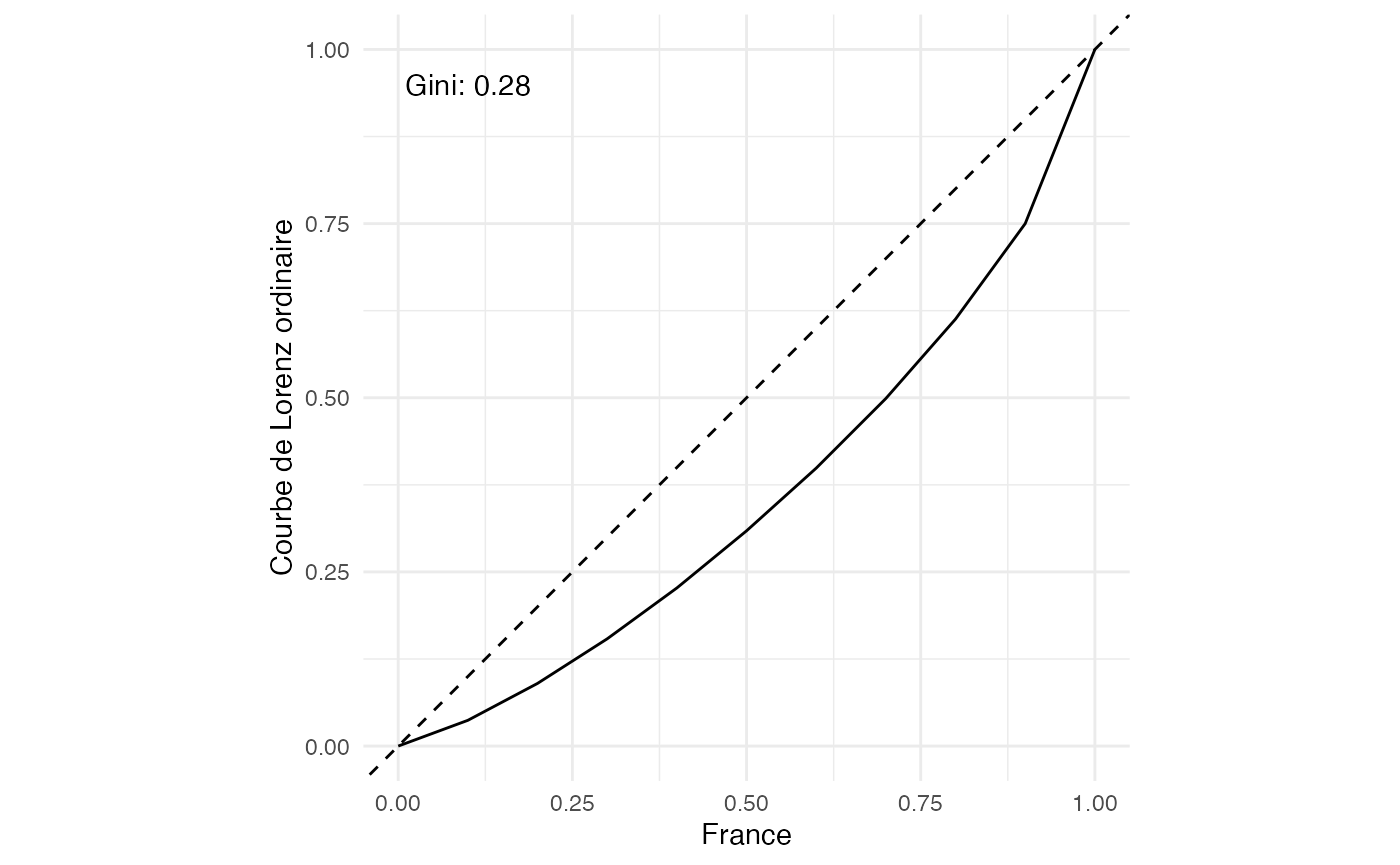
Représentations graphiques univariés
Histogramme
data3 <- rep(c(2,3.5,4.75,5.75,7,9,10.5,11.75),c(4,8,10,14,20,12,9,3))
table(data3)
#> data3
#>     2   3.5  4.75  5.75     7     9  10.5 11.75
#>     4     8    10    14    20    12     9     3
data4 <-rnorm(25,8,3)
layout(1:2)
oldpar <- par()
par(mar = c(2, 2, 1, 1) + 0.1, mgp=c(2,1,0))
histofre <- hist(data4,breaks=c(min(c(data4,1)),3,4,5.5,6,8,10,11,max(12.5,data4)),main="",freq=F,xlab="",ylab="",lwd=2)
histofre <- hist(data4,main="",breaks=8,freq=F,xlab="",ylab="",lwd=2,xlim=c(min(data4),max(data4)))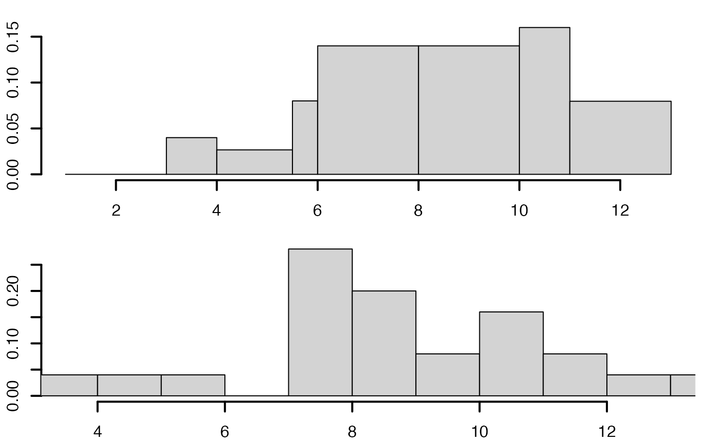
#suppressWarnings(par(oldpar))
pdf(file = paste(Chemin,"exemple_histo.pdf",sep=""),
    width = 6, height = 6, onefile = TRUE, family = "Helvetica",
    title = "europeSalaries boxplot", paper = "special")
layout(1:2)
oldpar <- par()
par(mar = c(0.2, 3, 0.2, 0.2) + 0.1, mgp = c(2, 1, 0))
histofre <- hist(data4,main="",breaks=8,freq=F,xlab="",ylab="",lwd=2,xlim=c(min(data4),max(data4)))
histofre <- hist(data4,breaks=c(min(c(data4,1)),3,4,5.5,6,8,10,11,max(12.5,data4)),main="",freq=F,xlab="",ylab="",lwd=2)
#suppressWarnings(par(oldpar))
dev.off()
#> agg_png
#>       2
Avec le package MASS.
layout(1:2)
oldpar <- par()
par(mar = c(2, 2, 1, 1) + 0.1, mgp=c(2,1,0))
truehist(data4,breaks=c(min(c(data4,1)),3,4,5.5,6,8,10,11,max(12.5,data4)),main="",freq=F,xlab="",ylab="",lwd=2)
#> Warning in plot.window(...): "freq" is not a graphical parameter
#> Warning in plot.xy(xy, type, ...): "freq" is not a graphical parameter
#> Warning in axis(side = side, at = at, labels = labels, ...): "freq" is not a
#> graphical parameter
#> Warning in axis(side = side, at = at, labels = labels, ...): "freq" is not a
#> graphical parameter
#> Warning in box(...): "freq" is not a graphical parameter
#> Warning in title(...): "freq" is not a graphical parameter
truehist(data4,main="",nbins=8,h=diff(range(data4))/7,xlab="",ylab="",lwd=2,xlim=c(min(data4),max(data4)))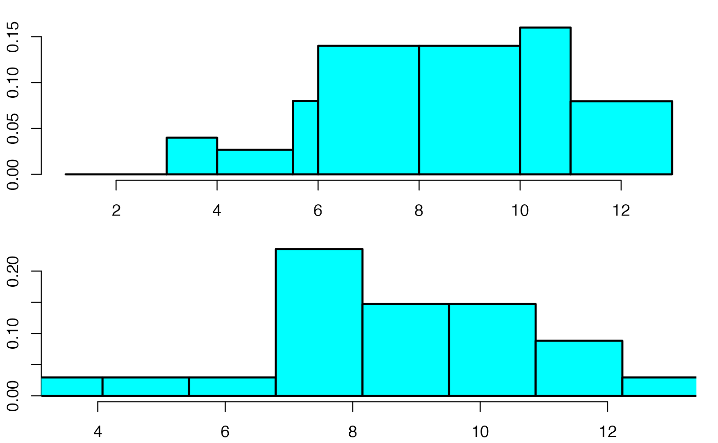
#suppressWarnings(par(oldpar))
pdf(file = paste(Chemin,"exemple_histo_MASS.pdf",sep=""),
    width = 6, height = 6, onefile = TRUE, family = "Helvetica",
    title = "europeSalaries boxplot", paper = "special")
layout(1:2)
oldpar <- par()
par(mar = c(2, 2, 1, 1) + 0.1, mgp=c(2,1,0))
truehist(data4,breaks=c(min(c(data4,1)),3,4,5.5,6,8,10,11,max(12.5,data4)),main="",freq=F,xlab="",ylab="",lwd=2)
#> Warning in plot.window(...): "freq" is not a graphical parameter
#> Warning in plot.xy(xy, type, ...): "freq" is not a graphical parameter
#> Warning in axis(side = side, at = at, labels = labels, ...): "freq" is not a
#> graphical parameter
#> Warning in axis(side = side, at = at, labels = labels, ...): "freq" is not a
#> graphical parameter
#> Warning in box(...): "freq" is not a graphical parameter
#> Warning in title(...): "freq" is not a graphical parameter
truehist(data4,main="",nbins=8,h=diff(range(data4))/7,xlab="",ylab="",lwd=2,xlim=c(min(data4),max(data4)))
#suppressWarnings(par(oldpar))
dev.off()
#> agg_png
#>       2
Par secteur de l’OCDE en 2020-Q3
data(Total_Secteur)
Total_Secteur
#>              Secteur        NameX  Effectif
#> 1                AGR  Agriculture  21143585
#> 2             CONSTR Construction  35197834
#> 3 INDUSwithoutCONSTR    Industrie  69941779
#> 4                MFG  Fabrication  64298386
#> 5               SERV     Services 368931820
NameX <- Total_Secteur$NameX
Effectif <- Total_Secteur$Effectif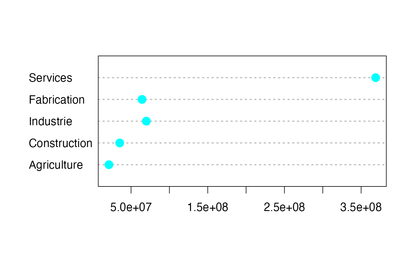
dotchart3(Effectif,labels=NameX,pch=19,col="#00FFFF")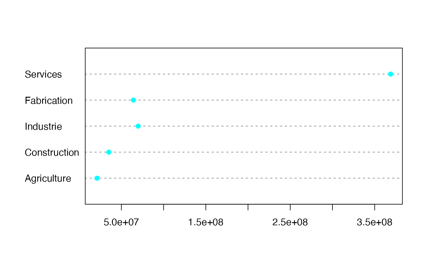
Chemin <- "~/Documents/Recherche/DeBoeck/Graphes/"
colmodel="cmyk"
pdf(file = paste(Chemin,"pointshoriz.pdf",sep=""),
    width = 8, height = 7, onefile = TRUE, family = "Helvetica",
    title = "Probability or cumulative distribution graphs", paper = "special", colormodel = colmodel)
par(mar = c(2, 2, 1, 1) + 0.1, mgp = c(2, 1, 0))
dotchart3(Effectif,labels=NameX,pch=19,col="#00FFFF",cex=1.6,cex.axis=1.2)
dev.off()
#> agg_png
#>       2

pdf(file = paste(Chemin,"pointshoriz_fre.pdf",sep=""),
    width = 8, height = 7, onefile = TRUE, family = "Helvetica",
    title = "Probability or cumulative distribution graphs", paper = "special", colormodel = colmodel)
par(mar = c(2, 2, 1, 1) + 0.1, mgp = c(2, 1, 0))
dotchart3(Effectif/sum(Effectif),labels=NameX,pch=19,col="#00FFFF",cex=1.6,cex.axis=1.2)
dev.off()
#> agg_png
#>       2
par(mar = c(2, 2, 1, 1) + 0.1, mgp = c(2, 1, 0))
pie(Effectif,labels=NameX,col=c("black","#00FFFF","black","#00FFFF"),density = c(rep(10,4),15),border=c("black","#00FFFF","black","#00FFFF"),cex=1.2)#,density = c(4*(4:1))
par(mar = c(2, 2, 1, 1) + 0.1, mgp = c(2, 1, 0))
#pie(Effectif,labels=NameX,col=c("#00000050","#00FFFF80","#00000050","#00FFFF80"),border=c("#00000050","#00FFFF80","#00000050","#00FFFF80"),cex=1.2)
par(mar = c(2, 2, 1, 1) + 0.1, mgp = c(2, 1, 0))
pie(Effectif,labels=NameX,col=c("black","#00FFFF","black","#00FFFF"),border=c("black","#00FFFF","black","#00FFFF"),cex=1.2)
pdf(file = paste(Chemin,"diagcircu.pdf",sep=""),
    width = 8, height = 7, onefile = TRUE, family = "Helvetica",
    title = "Probability or cumulative distribution graphs", paper = "special", colormodel = colmodel)
par(mar = c(2, 2, 1, 1) + 0.1, mgp = c(2, 1, 0))
pie(Effectif,labels=NameX,col=c("black","#00FFFF","black","#00FFFF","#FF00FF"),border=c("black","#00FFFF","black","#00FFFF"),cex=1.2)
dev.off()
#> agg_png
#>       2


pdf(file = paste(Chemin,"diagcircubis.pdf",sep=""),
    width = 8, height = 7, onefile = TRUE, family = "Helvetica",
    title = "Probability or cumulative distribution graphs", paper = "special", colormodel = colmodel)
par(mar = c(2, 2, 1, 1) + 0.1, mgp = c(2, 1, 0))
pie(Effectif,labels=NameX,col=c("black","#00FFFF","black","#00FFFF"),density = c(rep(10,4),15),border=c("black","#00FFFF","black","#00FFFF"),cex=1.2)#,density = c(4*(4:1))
dev.off()
#> agg_png
#>       2
NameXbar <- NameX
par(mar = c(8.1, 2, 1, 1) + 0.1, mgp = c(2, 1, 0))
barplot(Effectif,names.arg=NameXbar,col=c("black","#00FFFF","black","#00FFFF"),cex.axis=1.2,cex.names=1.2)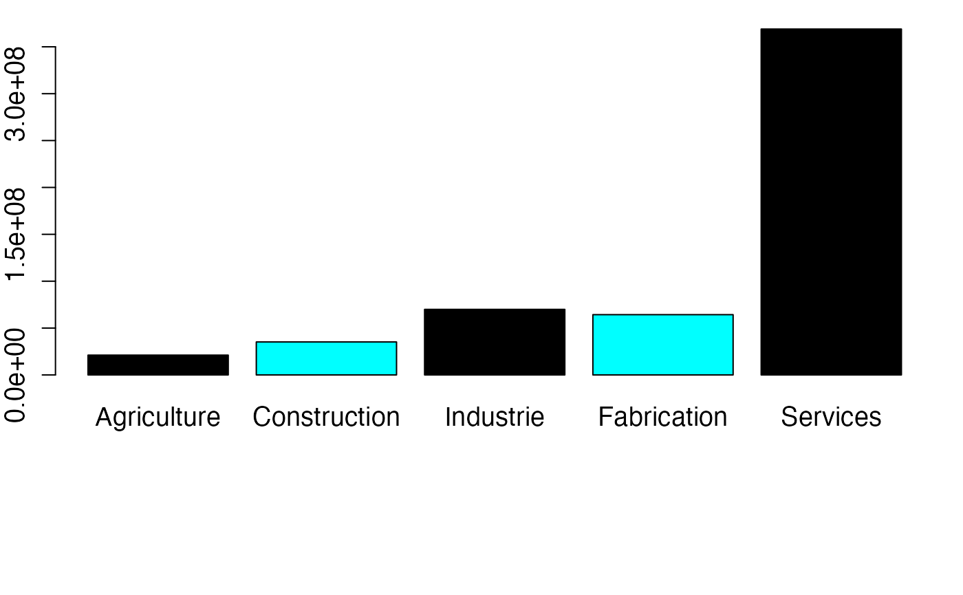
pdf(file = paste(Chemin,"barverti.pdf",sep=""),
    width = 8, height = 7, onefile = TRUE, family = "Helvetica",
    title = "Probability or cumulative distribution graphs", paper = "special", colormodel = colmodel)
par(mar = c(8.1, 2, 1, 1) + 0.1, mgp = c(2, 1, 0))
barplot(Effectif,names.arg=NameXbar,col=c("black","#00FFFF","black","#00FFFF"),las=3)
dev.off()
#> agg_png
#>       2

pdf(file = paste(Chemin,"barvertibis.pdf",sep=""),
    width = 8, height = 7, onefile = TRUE, family = "Helvetica",
    title = "Probability or cumulative distribution graphs", paper = "special", colormodel = colmodel)
par(mar = c(8.1, 2, 1, 1) + 0.1, mgp = c(2, 1, 0))
barplot(Effectif,names.arg=NameXbar,col=c("black","#00FFFF","black","#00FFFF"),density = 10,border=c("black","#00FFFF","black","#00FFFF"),cex.axis=1.2,las=3)
dev.off()
#> agg_png
#>       2

pdf(file = paste(Chemin,"barverti_fre.pdf",sep=""),
    width = 8, height = 7, onefile = TRUE, family = "Helvetica",
    title = "Probability or cumulative distribution graphs", paper = "special", colormodel = colmodel)
par(mar = c(8.1, 2, 1, 1) + 0.1, mgp = c(2, 1, 0))
barplot(Effectif/sum(Effectif),names.arg=NameXbar,col=c("black","#00FFFF","black","#00FFFF"),las=3)
dev.off()
#> agg_png
#>       2

pdf(file = paste(Chemin,"barvertibis_fre.pdf",sep=""),
    width = 8, height = 7, onefile = TRUE, family = "Helvetica",
    title = "Probability or cumulative distribution graphs", paper = "special", colormodel = colmodel)
par(mar = c(8.1, 2, 1, 1) + 0.1, mgp = c(2, 1, 0))
barplot(Effectif/sum(Effectif),names.arg=NameXbar,col=c("black","#00FFFF","black","#00FFFF"),density = 10,border=c("black","#00FFFF","black","#00FFFF"),cex.axis=1.2,las=3)
dev.off()
#> agg_png
#>       2
NameXbar <- NameX
par(mar = c(2, 8.1, 1, 1) + 0.1, mgp = c(2, 1, 0))
barplot(Effectif,names.arg=NameXbar,col=c("black","#00FFFF","black","#00FFFF"),cex.axis=1.2,cex.names=1.2,horiz=TRUE,las=1)
pdf(file = paste(Chemin,"barhoriz.pdf",sep=""),
    width = 8, height = 7, onefile = TRUE, family = "Helvetica",
    title = "Probability or cumulative distribution graphs", paper = "special", colormodel = colmodel)
par(mar = c(2, 8.1, 1, 1) + 0.1, mgp = c(2, 1, 0))
barplot(Effectif,names.arg=NameXbar,col=c("black","#00FFFF","black","#00FFFF"),horiz=TRUE,las=1)
dev.off()
#> agg_png
#>       2

pdf(file = paste(Chemin,"barhorizbis.pdf",sep=""),
    width = 8, height = 7, onefile = TRUE, family = "Helvetica",
    title = "Probability or cumulative distribution graphs", paper = "special", colormodel = colmodel)
par(mar = c(2, 8.1, 1, 1) + 0.1, mgp = c(2, 1, 0))
barplot(Effectif,names.arg=NameXbar,col=c("black","#00FFFF","black","#00FFFF"),density = 10,border=c("black","#00FFFF","black","#00FFFF"),cex.axis=1.2,horiz=TRUE,las=1)
dev.off()
#> agg_png
#>       2

pdf(file = paste(Chemin,"barhoriz_fre.pdf",sep=""),
    width = 8, height = 7, onefile = TRUE, family = "Helvetica",
    title = "Probability or cumulative distribution graphs", paper = "special", colormodel = colmodel)
par(mar = c(2, 8.1, 1, 1) + 0.1, mgp = c(2, 1, 0))
barplot(Effectif/sum(Effectif),names.arg=NameXbar,col=c("black","#00FFFF","black","#00FFFF"),horiz=TRUE,las=1)
dev.off()
#> agg_png
#>       2

pdf(file = paste(Chemin,"barhorizbis_fre.pdf",sep=""),
    width = 8, height = 7, onefile = TRUE, family = "Helvetica",
    title = "Probability or cumulative distribution graphs", paper = "special", colormodel = colmodel)
par(mar = c(2, 8.1, 1, 1) + 0.1, mgp = c(2, 1, 0))
barplot(Effectif/sum(Effectif),names.arg=NameXbar,col=c("black","#00FFFF","black","#00FFFF"),density = 10,border=c("black","#00FFFF","black","#00FFFF"),cex.axis=1.2,horiz=TRUE,las=1)
dev.off()
#> agg_png
#>       2

#suppressWarnings(par(oldpar))
Par pays de l’OCDE en 2020-Q3
data(Total_Pays)
Total_Pays
#>    NameX  Effectif
#> 1    AUT   5167648
#> 2    BEL   5721200
#> 3    CAN  21122321
#> 4    CHE   5568900
#> 5    CHL   8732089
#> 6    COL  22791085
#> 7    CZE   7015674
#> 8    DNK   3343269
#> 9    ESP  22701902
#> 10   EST    200241
#> 11   FIN   1154495
#> 12   FRA  31775373
#> 13   GBR  37353540
#> 14   GRC   4382010
#> 15   HUN   5787638
#> 16   IRL   2692289
#> 17   ISL     40222
#> 18   ISR   4366751
#> 19   ITA  28409214
#> 20   JPN  81977909
#> 21   KOR  33262656
#> 22   LTU   1647481
#> 23   LUX    316889
#> 24   LVA    253516
#> 25   NLD  10143660
#> 26   NOR   3114348
#> 27   NZL   3242630
#> 28   POL  21006175
#> 29   PRT   5902090
#> 30   SVK   3385346
#> 31   SVN   1275598
#> 32   SWE   5872257
#> 33   TUR  33604952
#> 34   USA 171209618
Effectif<-Total_Pays$Effectif
NameX<-Total_Pays$NameX
NameX2<-Total_Pays$NameX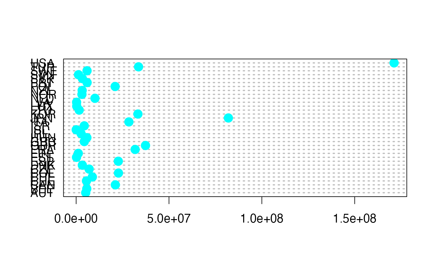
dotchart3(Effectif,labels=NameX2,pch=19,col="#00FFFF")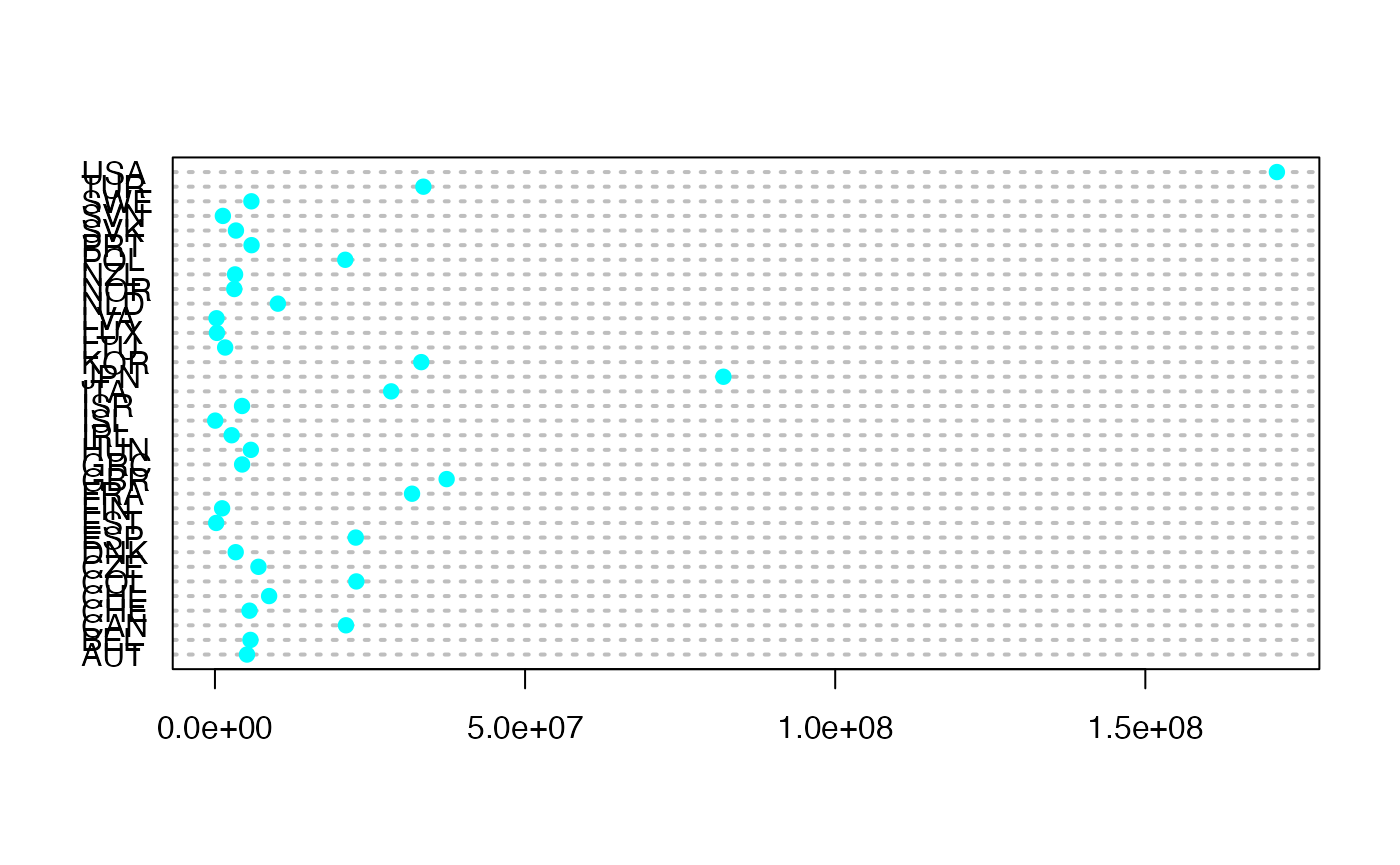
Chemin <- "~/Documents/Recherche/DeBoeck/Graphes/"
colmodel="cmyk"
pdf(file = paste(Chemin,"pointshoriz_app2.pdf",sep=""),
    width = 8, height = 7, onefile = TRUE, family = "Helvetica",
    title = "Probability or cumulative distribution graphs", paper = "special", colormodel = colmodel)
par(mar = c(2, 2, 1, 1) + 0.1, mgp = c(2, 1, 0))
dotchart3(Effectif,labels=NameX2,pch=19,col="#00FFFF",cex=1.6,cex.axis=1.2)
dev.off()
#> agg_png
#>       2


pdf(file = paste(Chemin,"pointshoriz_fre_app2.pdf",sep=""),
    width = 8, height = 7, onefile = TRUE, family = "Helvetica",
    title = "Probability or cumulative distribution graphs", paper = "special", colormodel = colmodel)
par(mar = c(2, 2, 1, 1) + 0.1, mgp = c(2, 1, 0))
dotchart3(Effectif/sum(Effectif),labels=NameX2,pch=19,col="#00FFFF",cex=1.6,cex.axis=1.2)
dev.off()
#> agg_png
#>       2
if(!("dplyr" %in% installed.packages())){install.packages("dplyr")}
library(dplyr)
#>
#> Attaching package: 'dplyr'
#> The following object is masked from 'package:MASS':
#>
#>     select
#> The following objects are masked from 'package:stats':
#>
#>     filter, lag
#> The following objects are masked from 'package:base':
#>
#>     intersect, setdiff, setequal, union
df <- data.frame(NameX2=rev(NameX2),
                 Effectif=rev(Effectif))
df <- df %>%
  mutate(text_y = cumsum(Effectif) - Effectif/2)
df
#>    NameX2  Effectif    text_y
#> 1     USA 171209618  85604809
#> 2     TUR  33604952 188012094
#> 3     SWE   5872257 207750698
#> 4     SVN   1275598 211324626
#> 5     SVK   3385346 213655098
#> 6     PRT   5902090 218298816
#> 7     POL  21006175 231752948
#> 8     NZL   3242630 243877351
#> 9     NOR   3114348 247055840
#> 10    NLD  10143660 253684844
#> 11    LVA    253516 258883432
#> 12    LUX    316889 259168634
#> 13    LTU   1647481 260150820
#> 14    KOR  33262656 277605888
#> 15    JPN  81977909 335226170
#> 16    ITA  28409214 390419732
#> 17    ISR   4366751 406807714
#> 18    ISL     40222 409011201
#> 19    IRL   2692289 410377456
#> 20    HUN   5787638 414617420
#> 21    GRC   4382010 419702244
#> 22    GBR  37353540 440570019
#> 23    FRA  31775373 475134476
#> 24    FIN   1154495 491599410
#> 25    EST    200241 492276778
#> 26    ESP  22701902 503727849
#> 27    DNK   3343269 516750434
#> 28    CZE   7015674 521929906
#> 29    COL  22791085 536833286
#> 30    CHL   8732089 552594872
#> 31    CHE   5568900 559745367
#> 32    CAN  21122321 573090978
#> 33    BEL   5721200 586512738
#> 34    AUT   5167648 591957162
if(!("ggrepel" %in% installed.packages())){install.packages("ggrepel")}
library(ggrepel)
theme_set(theme_void())
p1 <- ggplot(data = df, aes(x = "", y = Effectif, fill = NameX2)) +
  geom_bar(stat = "identity")+
geom_label_repel(aes(label = NameX2, y = text_y), nudge_x = 1.6)+
  coord_polar(theta = "y") + theme(legend.position='none')+
  theme(axis.title.x=element_blank(),
        axis.text.x=element_blank(),
        axis.ticks.x=element_blank())
p1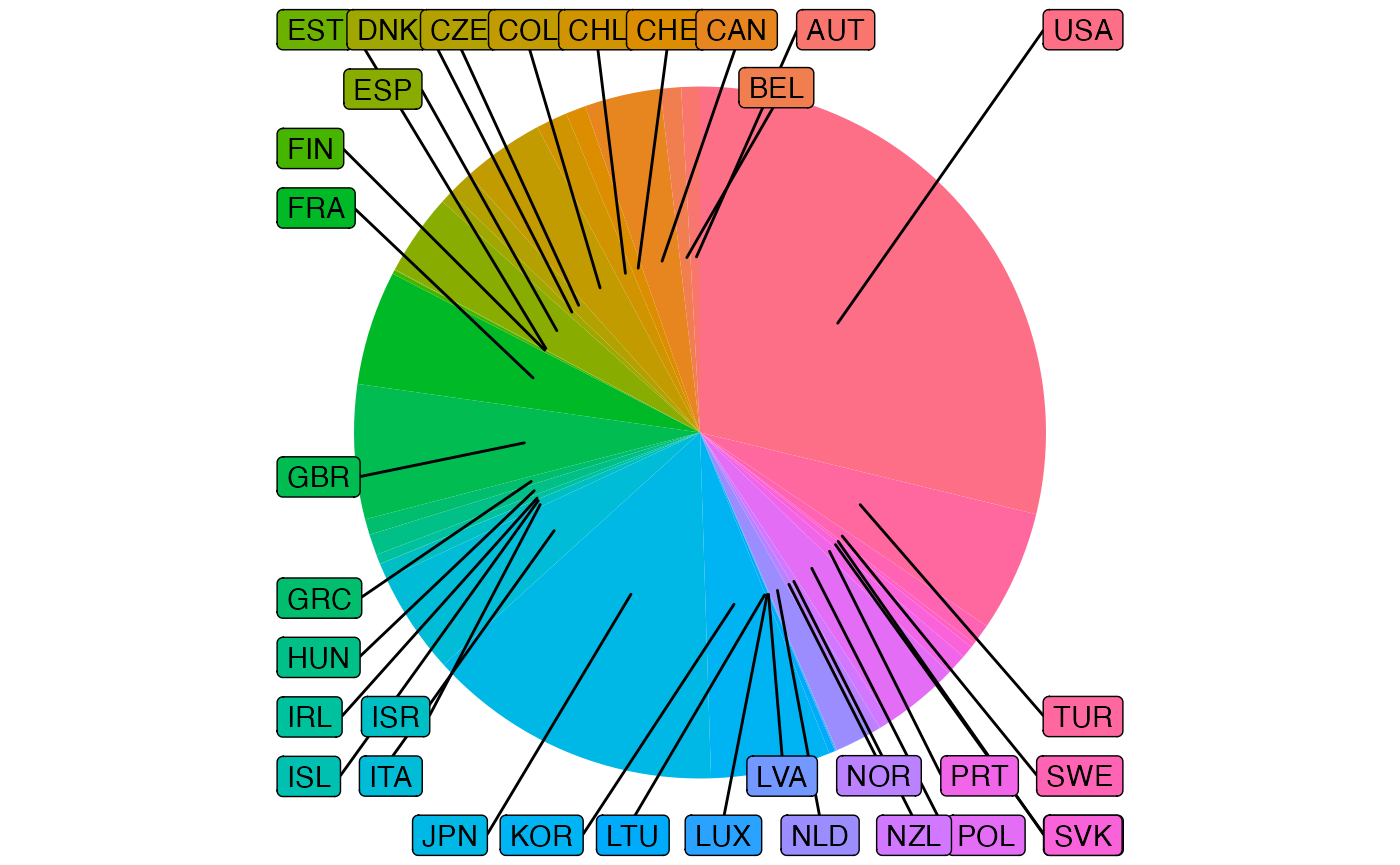
p1 + scale_fill_manual(values=rep(c(grey.colors(4)[c(2,4)]),17))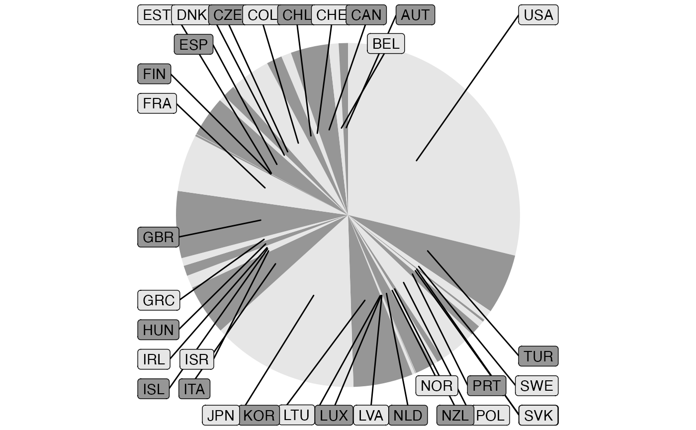
ggsave(filename = paste(Chemin,"diagcircu_app2_ggplot2.pdf",sep=""),
       width = 8, height = 7, onefile = TRUE, family = "Helvetica",
    title = "Probability or cumulative distribution graphs", paper = "special", colormodel = colmodel)
par(mar = c(2, 2, 1, 1) + 0.1, mgp = c(2, 1, 0))
pie(Effectif,labels=NameX2,col=c("black","#00FFFF","black","#00FFFF"),border=c("black","#00FFFF","black","#00FFFF"),cex=1.2)
pdf(file = paste(Chemin,"diagcircu_app2.pdf",sep=""),
    width = 8, height = 7, onefile = TRUE, family = "Helvetica",
    title = "Probability or cumulative distribution graphs", paper = "special", colormodel = colmodel)
par(mar = c(2, 2, 1, 1) + 0.1, mgp = c(2, 1, 0))
pie(Effectif,labels=NameX2,col=c("black","#00FFFF","black","#00FFFF"),border=c("black","#00FFFF","black","#00FFFF"),cex=1.2)
dev.off()
#> agg_png
#>       2
par(mar = c(2, 2, 1, 1) + 0.1, mgp = c(2, 1, 0))
pie(Effectif,labels=NameX2,col=c("black","#00FFFF","black","#00FFFF"),density = 10,border=c("black","#00FFFF","black","#00FFFF"),cex=1.2)#,density = c(4*(4:1))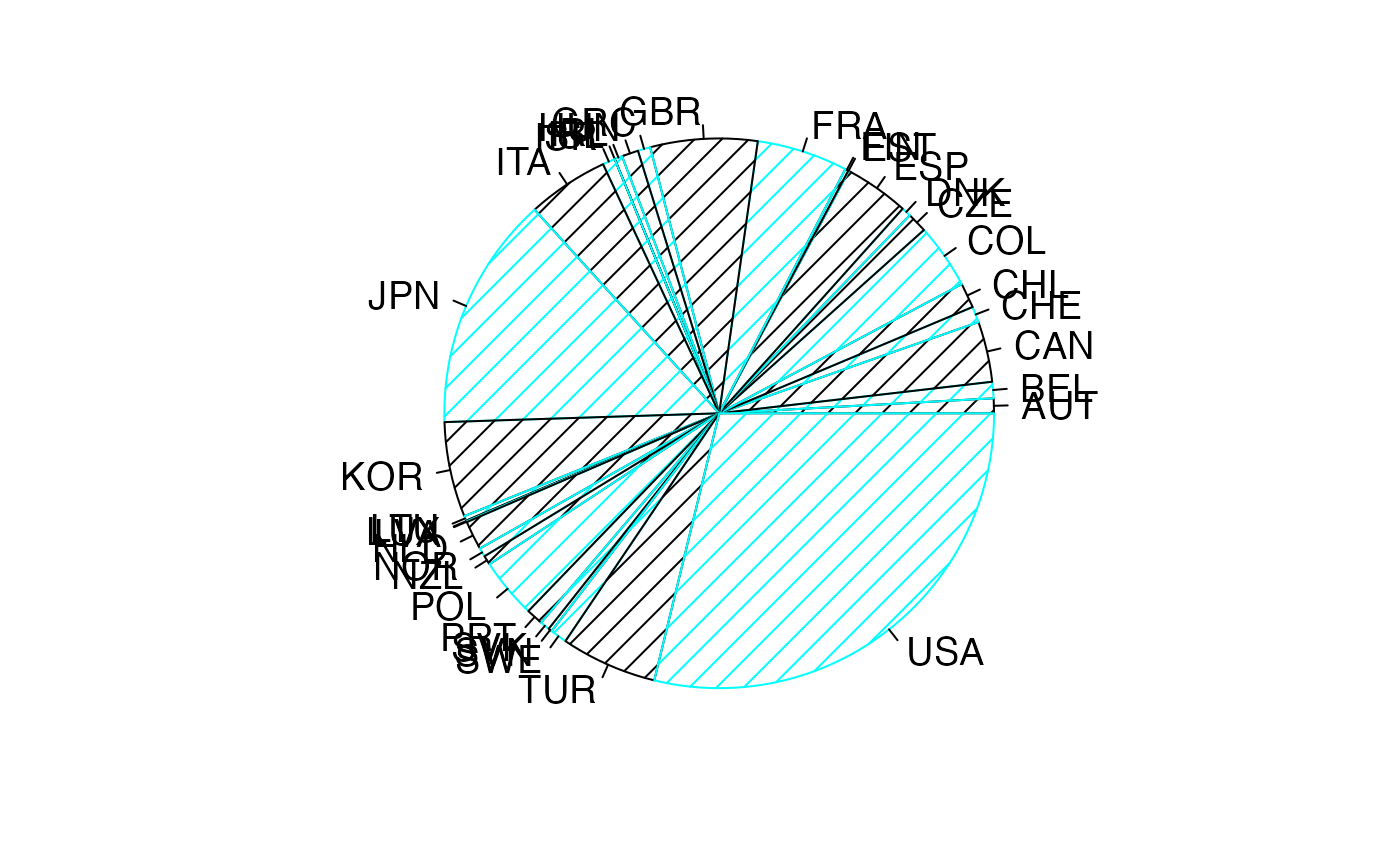
pdf(file = paste(Chemin,"diagcircubis_app2.pdf",sep=""),
    width = 8, height = 7, onefile = TRUE, family = "Helvetica",
    title = "Probability or cumulative distribution graphs", paper = "special", colormodel = colmodel)
par(mar = c(2, 2, 1, 1) + 0.1, mgp = c(2, 1, 0))
pie(Effectif,labels=NameX2,col=c("black","#00FFFF","black","#00FFFF"),density = 10,border=c("black","#00FFFF","black","#00FFFF"),cex=1.2)#,density = c(4*(4:1))
dev.off()
#> agg_png
#>       2
par(mar = c(6.3, 2, 1, 1) + 0.1, mgp = c(2, 1, 0))
NameXbar <- NameX2
barplot(Effectif,names.arg=NameXbar,col=c("black","#00FFFF","black","#00FFFF"),cex.axis=1.2,cex.names=1.2,las=3)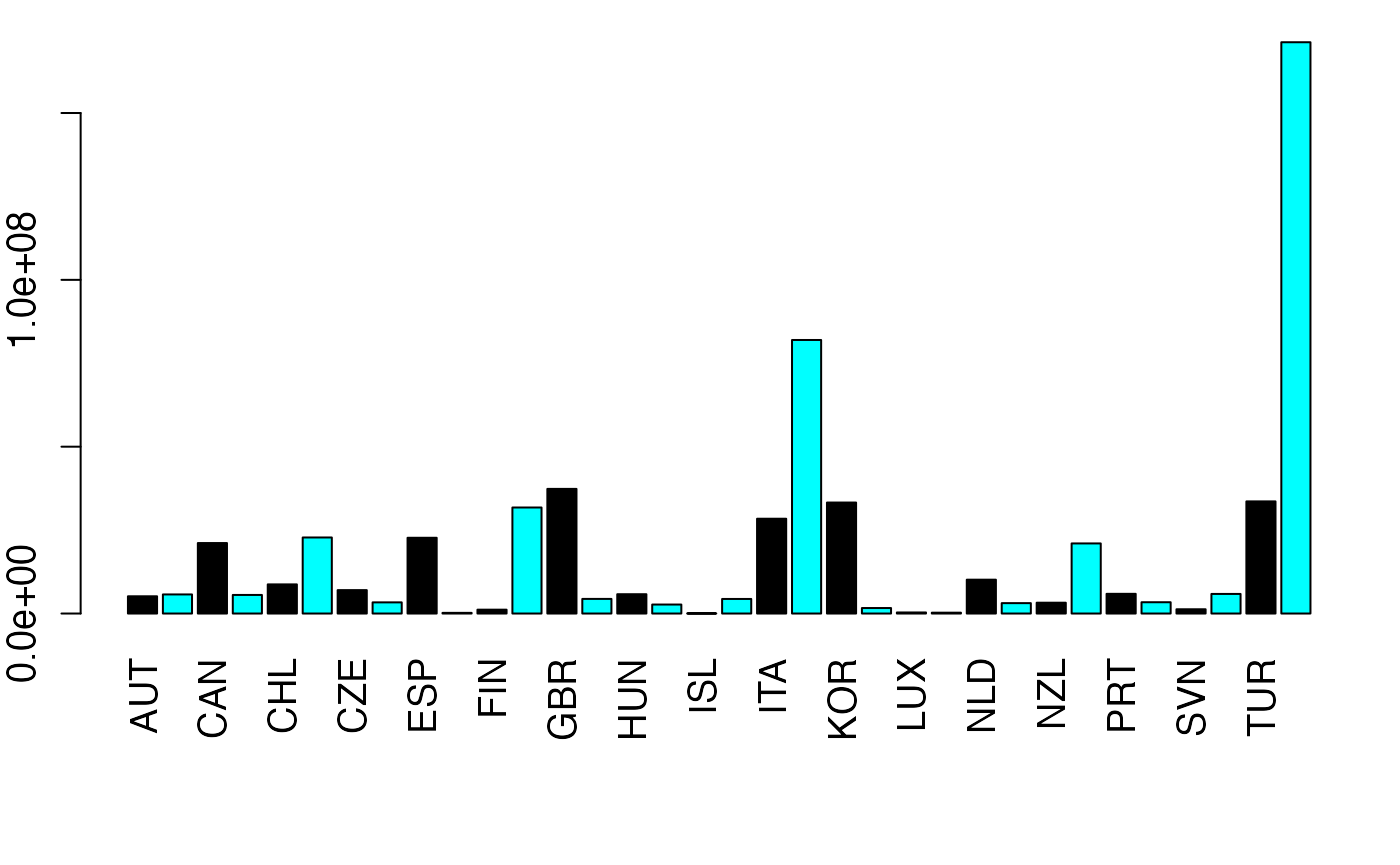
pdf(file = paste(Chemin,"barverti_app2.pdf",sep=""),
    width = 8, height = 7, onefile = TRUE, family = "Helvetica",
    title = "Probability or cumulative distribution graphs", paper = "special", colormodel = colmodel)
par(mar = c(6.3, 2, 1, 1) + 0.1, mgp = c(2, 1, 0))
barplot(Effectif,names.arg=NameXbar,col=c("black","#00FFFF","black","#00FFFF"),las=3)
dev.off()
#> agg_png
#>       2

pdf(file = paste(Chemin,"barvertibis_app2.pdf",sep=""),
    width = 8.1, height = 7, onefile = TRUE, family = "Helvetica",
    title = "Probability or cumulative distribution graphs", paper = "special", colormodel = colmodel)
par(mar = c(6.3, 2, 1, 1) + 0.1, mgp = c(2, 1, 0))
barplot(Effectif,names.arg=NameXbar,col=c("black","#00FFFF","black","#00FFFF"),density = 10,border=c("black","#00FFFF","black","#00FFFF"),cex.axis=1.2,las=3)
dev.off()
#> agg_png
#>       2

pdf(file = paste(Chemin,"barverti_fre_app2.pdf",sep=""),
    width = 8, height = 7, onefile = TRUE, family = "Helvetica",
    title = "Probability or cumulative distribution graphs", paper = "special", colormodel = colmodel)
par(mar = c(6.3, 2, 1, 1) + 0.1, mgp = c(2, 1, 0))
barplot(Effectif/sum(Effectif),names.arg=NameXbar,col=c("black","#00FFFF","black","#00FFFF"),las=3)
dev.off()
#> agg_png
#>       2

pdf(file = paste(Chemin,"barvertibis_fre_app2.pdf",sep=""),
    width = 8.1, height = 7, onefile = TRUE, family = "Helvetica",
    title = "Probability or cumulative distribution graphs", paper = "special", colormodel = colmodel)
par(mar = c(6.3, 2, 1, 1) + 0.1, mgp = c(2, 1, 0))
barplot(Effectif/sum(Effectif),names.arg=NameXbar,col=c("black","#00FFFF","black","#00FFFF"),density = 10,border=c("black","#00FFFF","black","#00FFFF"),cex.axis=1.2,las=3)
dev.off()
#> agg_png
#>       2
par(mar = c(2, 7, 1, 1) + 0.1, mgp = c(2, 1, 0))
NameXbar <- NameX2
barplot(Effectif,names.arg=NameXbar,col=c("black","#00FFFF","black","#00FFFF"),cex.axis=1.2,cex.names=1.2,las=1,horiz=TRUE)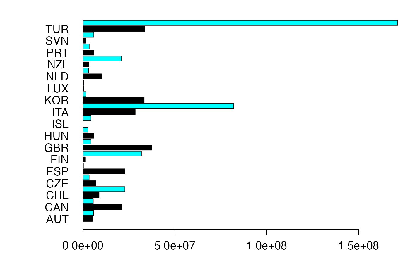
#suppressWarnings(par(oldpar))
pdf(file = paste(Chemin,"barhoriz_app2.pdf",sep=""),
    width = 8, height = 7, onefile = TRUE, family = "Helvetica",
    title = "Probability or cumulative distribution graphs", paper = "special", colormodel = colmodel)
par(mar = c(2, 7, 1, 1) + 0.1, mgp = c(2, 1, 0))
barplot(Effectif,names.arg=NameXbar,col=c("black","#00FFFF","black","#00FFFF"),las=1,horiz=TRUE)
dev.off()
#> agg_png
#>       2

pdf(file = paste(Chemin,"barhorizbis_app2.pdf",sep=""),
    width = 8.1, height = 7, onefile = TRUE, family = "Helvetica",
    title = "Probability or cumulative distribution graphs", paper = "special", colormodel = colmodel)
par(mar = c(2, 7, 1, 1) + 0.1, mgp = c(2, 1, 0))
barplot(Effectif,names.arg=NameXbar,col=c("black","#00FFFF","black","#00FFFF"),density = 10,border=c("black","#00FFFF","black","#00FFFF"),cex.axis=1.2,las=1,horiz=TRUE)
dev.off()
#> agg_png
#>       2

pdf(file = paste(Chemin,"barhoriz_fre_app2.pdf",sep=""),
    width = 8, height = 7, onefile = TRUE, family = "Helvetica",
    title = "Probability or cumulative distribution graphs", paper = "special", colormodel = colmodel)
par(mar = c(2, 7, 1, 1) + 0.1, mgp = c(2, 1, 0))
barplot(Effectif/sum(Effectif),names.arg=NameXbar,col=c("black","#00FFFF","black","#00FFFF"),las=1,horiz=TRUE)
dev.off()
#> agg_png
#>       2

pdf(file = paste(Chemin,"barhorizbis_fre_app2.pdf",sep=""),
    width = 8.1, height = 7, onefile = TRUE, family = "Helvetica",
    title = "Probability or cumulative distribution graphs", paper = "special", colormodel = colmodel)
par(mar = c(2, 7, 1, 1) + 0.1, mgp = c(2, 1, 0))
barplot(Effectif/sum(Effectif),names.arg=NameXbar,col=c("black","#00FFFF","black","#00FFFF"),density = 10,border=c("black","#00FFFF","black","#00FFFF"),cex.axis=1.2,las=1,horiz=TRUE)
dev.off()
#> agg_png
#>       2
Nombre de personnes par famille
data(Personnes_Foyer)
ni <- Personnes_Foyer$ni
xi <- Personnes_Foyer$xi

oldpar <- par()
par(mar = c(2, 2, 1, 1) + 0.1, mgp=c(2,1,0))
plot(xi,ni,type='h',xlab="",ylab="",lwd=2,xaxt="n")
axis(1, at = 1:6, labels = c(1:5,6))
#suppressWarnings(par(oldpar))
if(!("ggplot2" %in% installed.packages())){install.packages("ggplot2")}
library(ggplot2)
Diagramme en bâtons des effectifs
p1 <- ggplot(Personnes_Foyer) +
  geom_col(aes(y = ni, x = xi),width = .05)+
  xlab( expression(paste(x[i])))+
  ylab( expression(paste(n[i])))+
  scale_x_discrete(name =expression(paste(x[i])),
                 limits=c("1","2","3","4","5","6"))
p1
Chemin <- "~/Documents/Recherche/DeBoeck/Graphes/Sources/"
colmodel="cmyk"
ggsave(paste(Chemin,"batoneffnew.pdf",sep=""),
       width = 8, height = 7, onefile = TRUE, family = "Helvetica",
       title = "Diagramme en bâtons des effectifs",
       paper = "special", colormodel = colmodel)
oldpar <- par()
p1 <- ggplot(Personnes_Foyer) +
  geom_col(aes(y = ni/sum(ni), x = xi),width = .05)+
  xlab( expression(paste(x[i])))+
  ylab( expression(paste(n[i])))+
  scale_x_discrete(name =expression(paste(x[i])),
                   limits=c("1","2","3","4","5","6"))
p1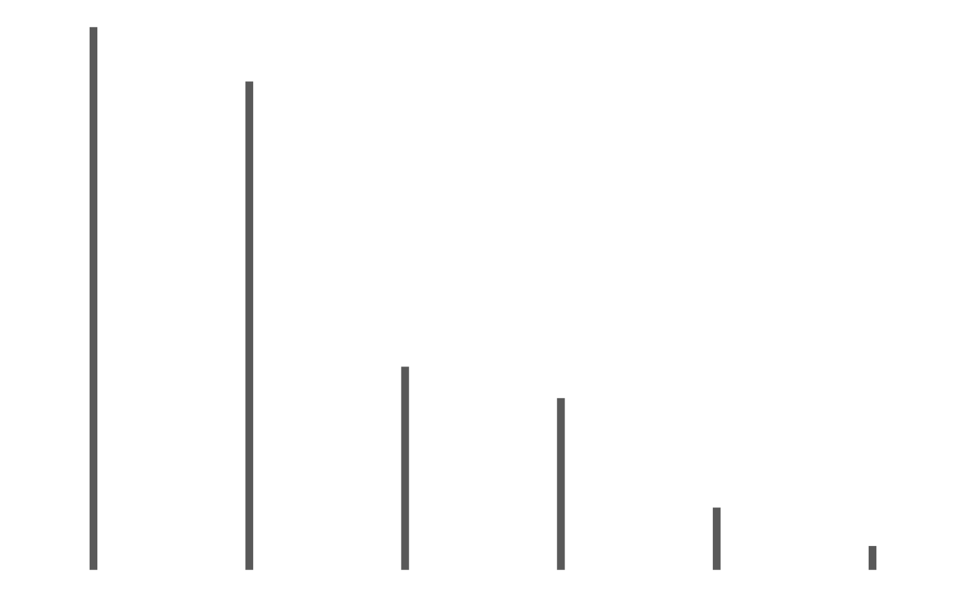
#suppressWarnings(par(oldpar))
ggsave(paste(Chemin,"batonfrenew.pdf",sep=""),
       width = 8, height = 7, onefile = TRUE, family = "Helvetica",
       title = "Probability or cumulative distribution graphs",
       paper = "special", colormodel = colmodel)
oldpar <- par()
ggplot(Personnes_Foyer, aes(x = xi)) +
  geom_ribbon(aes(ymin=0,ymax=ni,group=""),fill=I("gray80"))+
  geom_line(aes(y=ni,group=""), size=1, color=I("gray40")) +
  geom_pointrange(aes(ymin=0,ymax=ni,y=ni,group=""), size=1)+
  xlab( expression(paste(x[i])))+
  ylab( expression(paste(n[i])))+
  scale_x_discrete(name =expression(paste(x[i])),
                   limits=c("1","2","3","4","5","6"))
#> Warning: Using `size` aesthetic for lines was deprecated in ggplot2 3.4.0.
#> ℹ Please use `linewidth` instead.
#> This warning is displayed once every 8 hours.
#> Call `lifecycle::last_lifecycle_warnings()` to see where this warning was
#> generated.
#suppressWarnings(par(oldpar))
ggsave(paste(Chemin,"polyeffnew.pdf",sep=""),
       width = 8, height = 7, onefile = TRUE, family = "Helvetica",
       title = "Probability or cumulative distribution graphs",
       paper = "special", colormodel = colmodel)
oldpar <- par()
ggplot(Personnes_Foyer, aes(x = xi)) +
  geom_ribbon(aes(ymin=0,ymax=ni/sum(ni),group=""),fill=I("gray80"))+
  geom_line(aes(y=ni/sum(ni),group=""), size=1, color=I("gray40")) +
  geom_pointrange(aes(ymin=0,ymax=ni/sum(ni),y=ni/sum(ni),group=""), size=1)+
  xlab( expression(paste(x[i])))+
  ylab( expression(paste(n[i])))+
  scale_x_discrete(name =expression(paste(x[i])),
                   limits=c("1","2","3","4","5","6"))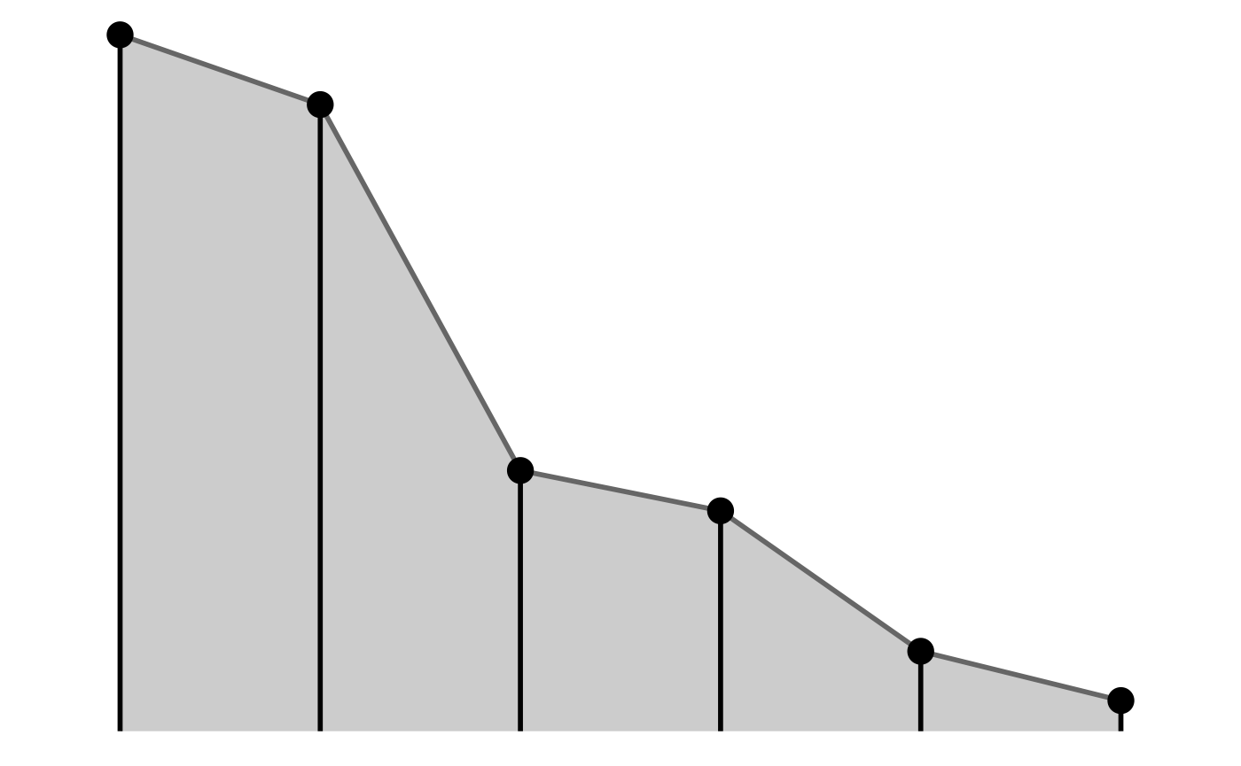
#suppressWarnings(par(oldpar))
ggsave(paste(Chemin,"polyfrenew.pdf",sep=""),
       width = 8, height = 7, onefile = TRUE, family = "Helvetica",
       title = "Probability or cumulative distribution graphs",
       paper = "special", colormodel = colmodel)
nisum <- rep(ni[1],length(ni))
for (iii in 2:length(ni))
{
nisum[iii] <- nisum[iii-1]+ni[iii]
}
data3<-data.frame(xi=xi,nisum=nisum)

oldpar <- par()
ggplot(data3, aes(x = xi)) +
  geom_ribbon(aes(ymin=0,ymax=nisum,group=""),fill=I("gray80"))+
  geom_line(aes(y=nisum,group=""), size=1, color=I("gray40")) +
  geom_pointrange(aes(ymin=0,ymax=nisum,y=nisum,group=""), size=1)+
  xlab( expression(paste(x[i])))+
  ylab( expression(paste(n[i])))+
  scale_x_discrete(name =expression(paste(x[i])),
                   limits=c("1","2","3","4","5","6"))
#suppressWarnings(par(oldpar))
ggsave(paste(Chemin,"polyeffcumnew.pdf",sep=""),
       width = 8, height = 7, onefile = TRUE, family = "Helvetica",
       title = "Probability or cumulative distribution graphs",
       paper = "special", colormodel = colmodel)
ggsave(paste(Chemin,"polyeffcumnew.svg",sep=""),device="svg",
       width = 8, height = 7)
data4<-data.frame(xi=xi,nifre=nisum/sum(ni))

oldpar <- par()
ggplot(data4, aes(x = xi)) +
  geom_ribbon(aes(ymin=0,ymax=nifre,group=""),fill=I("gray80"))+
  geom_line(aes(y=nifre,group=""), size=1, color=I("gray40")) +
  geom_pointrange(aes(ymin=0,ymax=nifre,y=nifre,group=""), size=1)+
  xlab( expression(paste(x[i])))+
  ylab( expression(paste(n[i])))+
  scale_x_discrete(name =expression(paste(x[i])),
                   limits=c("1","2","3","4","5","6"))
#> Warning: Using `size` aesthetic for lines was deprecated in ggplot2 3.4.0.
#> ℹ Please use `linewidth` instead.
#> This warning is displayed once every 8 hours.
#> Call `lifecycle::last_lifecycle_warnings()` to see where this warning was
#> generated.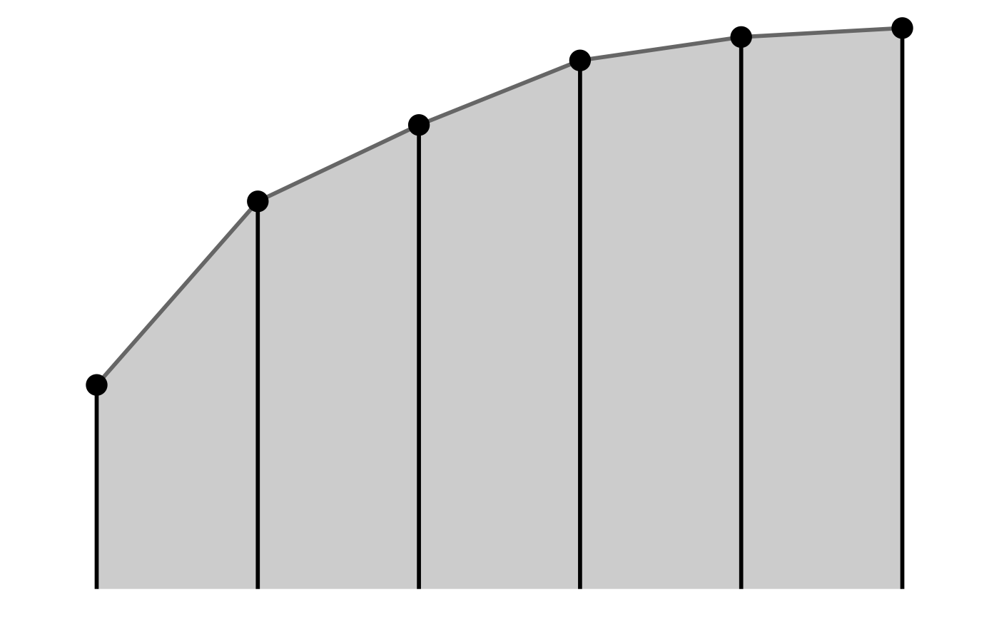
#suppressWarnings(par(oldpar))
ggsave(paste(Chemin,"frecumnew.pdf",sep=""),
       width = 8, height = 7, onefile = TRUE, family = "Helvetica",
       title = "Probability or cumulative distribution graphs",
       paper = "special", colormodel = colmodel)
p1 <- ggplot(data3) +
  geom_col(aes(y = nisum, x = xi),width = .05)+
  xlab( expression(paste(x[i])))+
  ylab( expression(paste(n[i])))+
  scale_x_discrete(name =expression(paste(x[i])),
                   limits=c("1","2","3","4","5","6"))
p1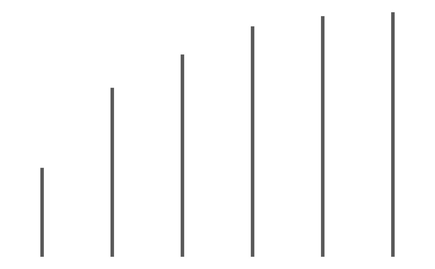
Population du Canada
data(AgevsProter_Canada_full)
valeursall <- margin.table(as.matrix(AgevsProter_Canada_full[,-1]),1)
valeurs <- valeursall[-length(valeursall)]
valeurs
#>   0 à 4 ans   5 à 9 ans 10 à 14 ans 15 à 19 ans 20 à 24 ans 25 à 29 ans
#>     1901542     2021227     2045914     2073871     2453892     2617164
#> 30 à 34 ans 35 à 39 ans 40 à 44 ans 45 à 49 ans 50 à 54 ans 55 à 59 ans
#>     2632781     2600529     2432821     2354362     2409701     2701791
#> 60 à 64 ans 65 à 69 ans 70 à 74 ans 75 à 79 ans 80 à 84 ans 85 à 89 ans
#>     2517902     2127557     1753443     1197845      798753      511048
#> 90 à 94 ans 95 à 99 ans
#>      245878       73725
centres <- c(5*(0:19)+2.5)
limites <- 5*(0:20)


oldpar <- par()


data3 <- rep(centres,valeurs)
table(data3)
#> data3
#>     2.5     7.5    12.5    17.5    22.5    27.5    32.5    37.5    42.5    47.5
#> 1901542 2021227 2045914 2073871 2453892 2617164 2632781 2600529 2432821 2354362
#>    52.5    57.5    62.5    67.5    72.5    77.5    82.5    87.5    92.5    97.5
#> 2409701 2701791 2517902 2127557 1753443 1197845  798753  511048  245878   73725

oldpar <- par()
par(mar = c(2, 2, 1, 1) + 0.1, mgp=c(2,1,0))
histofre <- hist(data3,breaks=limites,main="",freq=T,xlab="",ylab="",lwd=2,density=10)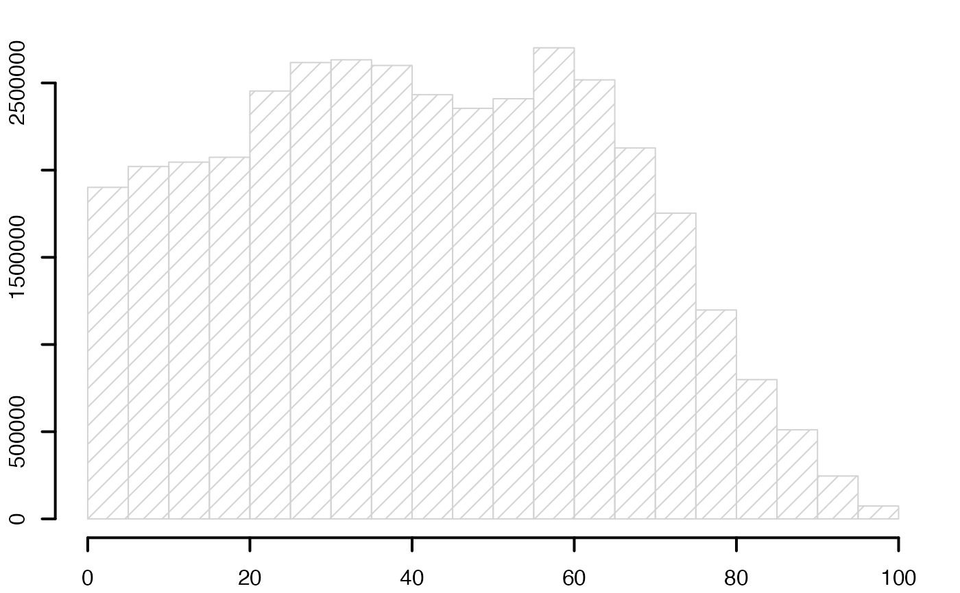
#suppressWarnings(par(oldpar))
Chemin <- "~/Documents/Recherche/DeBoeck/Graphes/Sources/"
colmodel="cmyk"
pdf(file = paste(Chemin,"histoeffnew.pdf",sep=""),
    width = 8, height = 7, onefile = TRUE, family = "Helvetica",
    title = "Probability or cumulative distribution graphs", paper = "special", colormodel = colmodel)
par(mar = c(2, 2, 1, 1) + 0.1, mgp = c(2, 1, 0))
histofre <- hist(data3,breaks=limites,main="",freq=T,xlab="",ylab="",lwd=2,density=10)
dev.off()
#> agg_png
#>       2
oldpar <- par()
par(mar = c(2, 2, 1, 1) + 0.1, mgp=c(2,1,0))
histofre <- hist(data3,breaks=limites,main="",freq=F,xlab="",ylab="",lwd=2,density=10)
#suppressWarnings(par(oldpar))
pdf(file = paste(Chemin,"histofrenew.pdf",sep=""),
    width = 8, height = 7, onefile = TRUE, family = "Helvetica",
    title = "Probability or cumulative distribution graphs", paper = "special", colormodel = colmodel)
par(mar = c(2, 2, 1, 1) + 0.1, mgp = c(2, 1, 0))
histofre <- hist(data3,breaks=limites,main="",freq=F,xlab="",ylab="",lwd=2,density=10)
dev.off()
#> agg_png
#>       2
oldpar <- par()
par(mar = c(2, 2, 1, 1) + 0.1, mgp=c(2,1,0))
histofre <- hist(data3,breaks=limites,main="",freq=F,xlab="",ylab="",lwd=2,density=10)
segments(histofre$mids[-length(histofre$mids)],histofre$density[-length(histofre$density)],histofre$mids[-1],histofre$density[-1],lwd=2,col="#00FFFF")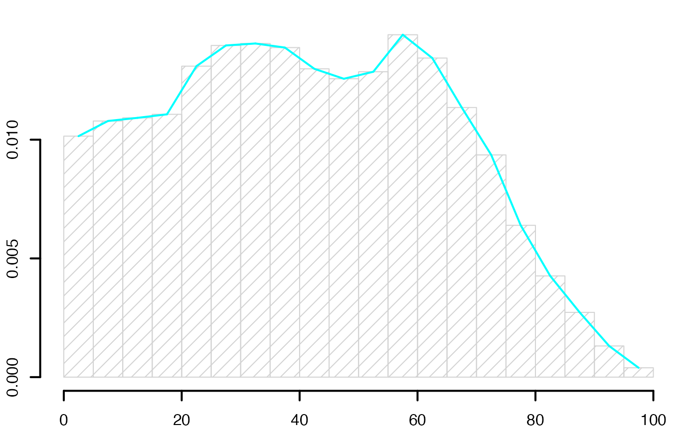
#suppressWarnings(par(oldpar))
pdf(file = paste(Chemin,"histopolfrenew.pdf",sep=""),
    width = 8, height = 7, onefile = TRUE, family = "Helvetica",
    title = "Probability or cumulative distribution graphs", paper = "special", colormodel = colmodel)
par(mar = c(2, 2, 1, 1) + 0.1, mgp = c(2, 1, 0))
histofre <- hist(data3,breaks=limites,main="",freq=F,xlab="",ylab="",lwd=2,density=10)
segments(histofre$mids[-length(histofre$mids)],histofre$density[-length(histofre$density)],histofre$mids[-1],histofre$density[-1],lwd=2,col="#00FFFF")
dev.off()
#> agg_png
#>       2
nihistsum <- rep(0,length(valeurs))
for (iii in 2:(length(valeurs)+1))
{
nihistsum[iii] <- nihistsum[iii-1]+(valeurs)[iii-1]
}

data4 <- rep(centres,cumsum(valeurs))
table(data4)
#> data4
#>      2.5      7.5     12.5     17.5     22.5     27.5     32.5     37.5
#>  1901542  3922769  5968683  8042554 10496446 13113610 15746391 18346920
#>     42.5     47.5     52.5     57.5     62.5     67.5     72.5     77.5
#> 20779741 23134103 25543804 28245595 30763497 32891054 34644497 35842342
#>     82.5     87.5     92.5     97.5
#> 36641095 37152143 37398021 37471746

oldpar <- par()
par(mar = c(2, 2, 1, 1) + 0.1, mgp=c(2,1,0))
histofrecum <- hist(data4,breaks=limites,main="",freq=T,xlab="",ylab="",lwd=2,yaxt="n",density=10)
axis(2,at=c(0,.2,.4,.6,.8,1)*max(histofrecum$counts),labels=format(c(0,.2,.4,.6,.8,1)*max(histofrecum$counts),scientific = TRUE,digits = 3),lwd=2)
#suppressWarnings(par(oldpar))
pdf(file = paste(Chemin,"histoeffcumnew.pdf",sep=""),
    width = 8, height = 7, onefile = TRUE, family = "Helvetica",
    title = "Probability or cumulative distribution graphs", paper = "special", colormodel = colmodel)
par(mar = c(2, 2, 1, 1) + 0.1, mgp = c(2, 1, 0))
histofrecum <- hist(data4,breaks=limites,main="",freq=T,xlab="",ylab="",lwd=2,yaxt="n",density=10)
axis(2,at=c(0,.2,.4,.6,.8,1)*max(histofrecum$counts),labels=round(c(0,.2,.4,.6,.8,1)*max(histofrecum$counts)),lwd=2)
dev.off()
#> agg_png
#>       2
oldpar <- par()
par(mar = c(2, 2, 1, 1) + 0.1, mgp=c(2,1,0))
histofrecum <- hist(data4,breaks=limites,main="",freq=F,xlab="",ylab="",lwd=2,yaxt="n",density=10)
axis(2,at=c(0,.2,.4,.6,.8,1)*max(histofrecum$dens),labels=c(0,.2,.4,.6,.8,1),lwd=2)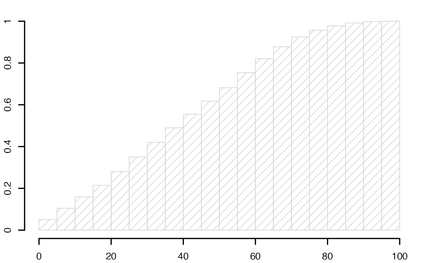
#suppressWarnings(par(oldpar))
pdf(file = paste(Chemin,"histofrecumnew.pdf",sep=""),
    width = 8, height = 7, onefile = TRUE, family = "Helvetica",
    title = "Probability or cumulative distribution graphs", paper = "special", colormodel = colmodel)
par(mar = c(2, 2, 1, 1) + 0.1, mgp = c(2, 1, 0))
histofrecum <- hist(data4,breaks=limites,main="",freq=F,xlab="",ylab="",lwd=2,yaxt="n",density=10)
axis(2,at=c(0,.2,.4,.6,.8,1)*max(histofrecum$dens),labels=c(0,.2,.4,.6,.8,1),lwd=2)
dev.off()
#> agg_png
#>       2
oldpar <- par()
par(mar = c(2, 2, 1, 1) + 0.1, mgp=c(2,1,0))
histofrecum <- hist(data4,breaks=limites,main="",freq=F,xlab="",ylab="",lwd=2,yaxt="n",density=10)
segments(histofrecum$mids[-length(histofrecum$mids)],histofrecum$density[-length(histofrecum$mids)],histofrecum$mids[-1],histofrecum$density[-1],lwd=2,col="#00FFFF")
axis(2,at=c(0,.2,.4,.6,.8,1)*max(histofrecum$dens),labels=c(0,.2,.4,.6,.8,1),lwd=2)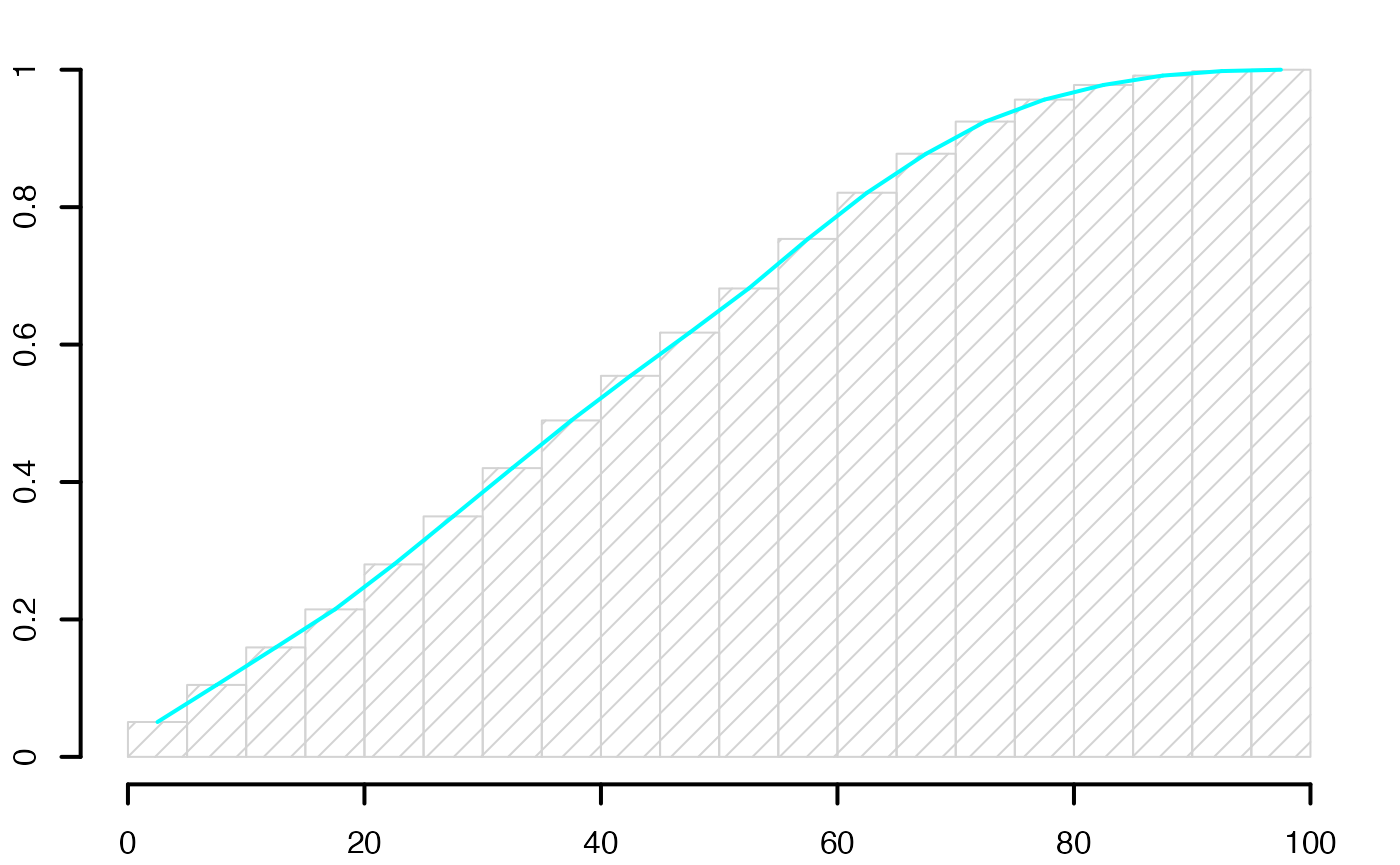
#suppressWarnings(par(oldpar))
pdf(file = paste(Chemin,"histopolfrecumnew.pdf",sep=""),
    width = 8, height = 7, onefile = TRUE, family = "Helvetica",
    title = "Probability or cumulative distribution graphs", paper = "special", colormodel = colmodel)
par(mar = c(2, 2, 1, 1) + 0.1, mgp = c(2, 1, 0))
histofrecum <- hist(data4,breaks=limites,main="",freq=F,xlab="",ylab="",lwd=2,yaxt="n",density=10)
segments(histofrecum$mids[-length(histofrecum$mids)],histofrecum$density[-length(histofrecum$mids)],histofrecum$mids[-1],histofrecum$density[-1],lwd=2,col="#00FFFF")
axis(2,at=c(0,.2,.4,.6,.8,1)*max(histofrecum$dens),labels=c(0,.2,.4,.6,.8,1),lwd=2)
dev.off()
#> agg_png
#>       2
Bonus : Sièges Voix
data(Sieges_Voix)
str(Sieges_Voix)
#> 'data.frame': 27 obs. of 4 variables:
#> $ Etats.Membres : chr "Allemagne" "Autriche" "Belgique" "Bulgarie" ...
#> $ Date.entrée : int 1957 1995 1957 2007 2004 1973 1986 2004 1995 1957 ...
#> $ Sièges.au.parlement: int 99 18 24 0 6 14 54 6 14 78 ...
#> $ Voix.au.conseil : int 29 10 12 0 4 7 27 4 7 29 ...
summary(Sieges_Voix)
#> Etats.Membres Date.entrée Sièges.au.parlement Voix.au.conseil
#> Length:27 Min. :1957 Min. : 0.00 Min. : 0.00
#> Class :character 1st Qu.:1973 1st Qu.: 8.00 1st Qu.: 4.00
#> Mode :character Median :1995 Median :18.00 Median :10.00
#> Mean :1987 Mean :27.11 Mean :11.89
#> 3rd Qu.:2004 3rd Qu.:25.50 3rd Qu.:12.50
#> Max. :2007 Max. :99.00 Max. :29.00
NameX <- Sieges_Voix$Etats.Membres
NombreSieges <- Sieges_Voix$Sièges.au.parlement
NombreVoix <- Sieges_Voix$Voix.au.conseil
NameXX <- names(table(Sieges_Voix$Date.entrée))
NombreAnnees <- as.vector(table(Sieges_Voix$Date.entrée))
names(NombreSieges) <- NameX
NombreSieges
#> Allemagne Autriche Belgique Bulgarie
#> 99 18 24 0
#> Chypre Danemark Espagne Estonie
#> 6 14 54 6
#> Finlande France Grèce Hongrie
#> 14 78 24 24
#> Irlande Italie Lettonie Lituanie
#> 13 78 9 13
#> Luxembourg Malte Pays-Bas Pologne
#> 6 5 27 54
#> Portugal République Tchèque Roumanie Royaume-Uni
#> 24 24 0 78
#> Slovaquie Slovénie Suède
#> 14 7 19
rep(NameX,NombreSieges)
#> [1] "Allemagne" "Allemagne" "Allemagne"
#> [4] "Allemagne" "Allemagne" "Allemagne"
#> [7] "Allemagne" "Allemagne" "Allemagne"
#> [10] "Allemagne" "Allemagne" "Allemagne"
#> [13] "Allemagne" "Allemagne" "Allemagne"
#> [16] "Allemagne" "Allemagne" "Allemagne"
#> [19] "Allemagne" "Allemagne" "Allemagne"
#> [22] "Allemagne" "Allemagne" "Allemagne"
#> [25] "Allemagne" "Allemagne" "Allemagne"
#> [28] "Allemagne" "Allemagne" "Allemagne"
#> [31] "Allemagne" "Allemagne" "Allemagne"
#> [34] "Allemagne" "Allemagne" "Allemagne"
#> [37] "Allemagne" "Allemagne" "Allemagne"
#> [40] "Allemagne" "Allemagne" "Allemagne"
#> [43] "Allemagne" "Allemagne" "Allemagne"
#> [46] "Allemagne" "Allemagne" "Allemagne"
#> [49] "Allemagne" "Allemagne" "Allemagne"
#> [52] "Allemagne" "Allemagne" "Allemagne"
#> [55] "Allemagne" "Allemagne" "Allemagne"
#> [58] "Allemagne" "Allemagne" "Allemagne"
#> [61] "Allemagne" "Allemagne" "Allemagne"
#> [64] "Allemagne" "Allemagne" "Allemagne"
#> [67] "Allemagne" "Allemagne" "Allemagne"
#> [70] "Allemagne" "Allemagne" "Allemagne"
#> [73] "Allemagne" "Allemagne" "Allemagne"
#> [76] "Allemagne" "Allemagne" "Allemagne"
#> [79] "Allemagne" "Allemagne" "Allemagne"
#> [82] "Allemagne" "Allemagne" "Allemagne"
#> [85] "Allemagne" "Allemagne" "Allemagne"
#> [88] "Allemagne" "Allemagne" "Allemagne"
#> [91] "Allemagne" "Allemagne" "Allemagne"
#> [94] "Allemagne" "Allemagne" "Allemagne"
#> [97] "Allemagne" "Allemagne" "Allemagne"
#> [100] "Autriche" "Autriche" "Autriche"
#> [103] "Autriche" "Autriche" "Autriche"
#> [106] "Autriche" "Autriche" "Autriche"
#> [109] "Autriche" "Autriche" "Autriche"
#> [112] "Autriche" "Autriche" "Autriche"
#> [115] "Autriche" "Autriche" "Autriche"
#> [118] "Belgique" "Belgique" "Belgique"
#> [121] "Belgique" "Belgique" "Belgique"
#> [124] "Belgique" "Belgique" "Belgique"
#> [127] "Belgique" "Belgique" "Belgique"
#> [130] "Belgique" "Belgique" "Belgique"
#> [133] "Belgique" "Belgique" "Belgique"
#> [136] "Belgique" "Belgique" "Belgique"
#> [139] "Belgique" "Belgique" "Belgique"
#> [142] "Chypre" "Chypre" "Chypre"
#> [145] "Chypre" "Chypre" "Chypre"
#> [148] "Danemark" "Danemark" "Danemark"
#> [151] "Danemark" "Danemark" "Danemark"
#> [154] "Danemark" "Danemark" "Danemark"
#> [157] "Danemark" "Danemark" "Danemark"
#> [160] "Danemark" "Danemark" "Espagne"
#> [163] "Espagne" "Espagne" "Espagne"
#> [166] "Espagne" "Espagne" "Espagne"
#> [169] "Espagne" "Espagne" "Espagne"
#> [172] "Espagne" "Espagne" "Espagne"
#> [175] "Espagne" "Espagne" "Espagne"
#> [178] "Espagne" "Espagne" "Espagne"
#> [181] "Espagne" "Espagne" "Espagne"
#> [184] "Espagne" "Espagne" "Espagne"
#> [187] "Espagne" "Espagne" "Espagne"
#> [190] "Espagne" "Espagne" "Espagne"
#> [193] "Espagne" "Espagne" "Espagne"
#> [196] "Espagne" "Espagne" "Espagne"
#> [199] "Espagne" "Espagne" "Espagne"
#> [202] "Espagne" "Espagne" "Espagne"
#> [205] "Espagne" "Espagne" "Espagne"
#> [208] "Espagne" "Espagne" "Espagne"
#> [211] "Espagne" "Espagne" "Espagne"
#> [214] "Espagne" "Espagne" "Estonie"
#> [217] "Estonie" "Estonie" "Estonie"
#> [220] "Estonie" "Estonie" "Finlande"
#> [223] "Finlande" "Finlande" "Finlande"
#> [226] "Finlande" "Finlande" "Finlande"
#> [229] "Finlande" "Finlande" "Finlande"
#> [232] "Finlande" "Finlande" "Finlande"
#> [235] "Finlande" "France" "France"
#> [238] "France" "France" "France"
#> [241] "France" "France" "France"
#> [244] "France" "France" "France"
#> [247] "France" "France" "France"
#> [250] "France" "France" "France"
#> [253] "France" "France" "France"
#> [256] "France" "France" "France"
#> [259] "France" "France" "France"
#> [262] "France" "France" "France"
#> [265] "France" "France" "France"
#> [268] "France" "France" "France"
#> [271] "France" "France" "France"
#> [274] "France" "France" "France"
#> [277] "France" "France" "France"
#> [280] "France" "France" "France"
#> [283] "France" "France" "France"
#> [286] "France" "France" "France"
#> [289] "France" "France" "France"
#> [292] "France" "France" "France"
#> [295] "France" "France" "France"
#> [298] "France" "France" "France"
#> [301] "France" "France" "France"
#> [304] "France" "France" "France"
#> [307] "France" "France" "France"
#> [310] "France" "France" "France"
#> [313] "France" "Grèce" "Grèce"
#> [316] "Grèce" "Grèce" "Grèce"
#> [319] "Grèce" "Grèce" "Grèce"
#> [322] "Grèce" "Grèce" "Grèce"
#> [325] "Grèce" "Grèce" "Grèce"
#> [328] "Grèce" "Grèce" "Grèce"
#> [331] "Grèce" "Grèce" "Grèce"
#> [334] "Grèce" "Grèce" "Grèce"
#> [337] "Grèce" "Hongrie" "Hongrie"
#> [340] "Hongrie" "Hongrie" "Hongrie"
#> [343] "Hongrie" "Hongrie" "Hongrie"
#> [346] "Hongrie" "Hongrie" "Hongrie"
#> [349] "Hongrie" "Hongrie" "Hongrie"
#> [352] "Hongrie" "Hongrie" "Hongrie"
#> [355] "Hongrie" "Hongrie" "Hongrie"
#> [358] "Hongrie" "Hongrie" "Hongrie"
#> [361] "Hongrie" "Irlande" "Irlande"
#> [364] "Irlande" "Irlande" "Irlande"
#> [367] "Irlande" "Irlande" "Irlande"
#> [370] "Irlande" "Irlande" "Irlande"
#> [373] "Irlande" "Irlande" "Italie"
#> [376] "Italie" "Italie" "Italie"
#> [379] "Italie" "Italie" "Italie"
#> [382] "Italie" "Italie" "Italie"
#> [385] "Italie" "Italie" "Italie"
#> [388] "Italie" "Italie" "Italie"
#> [391] "Italie" "Italie" "Italie"
#> [394] "Italie" "Italie" "Italie"
#> [397] "Italie" "Italie" "Italie"
#> [400] "Italie" "Italie" "Italie"
#> [403] "Italie" "Italie" "Italie"
#> [406] "Italie" "Italie" "Italie"
#> [409] "Italie" "Italie" "Italie"
#> [412] "Italie" "Italie" "Italie"
#> [415] "Italie" "Italie" "Italie"
#> [418] "Italie" "Italie" "Italie"
#> [421] "Italie" "Italie" "Italie"
#> [424] "Italie" "Italie" "Italie"
#> [427] "Italie" "Italie" "Italie"
#> [430] "Italie" "Italie" "Italie"
#> [433] "Italie" "Italie" "Italie"
#> [436] "Italie" "Italie" "Italie"
#> [439] "Italie" "Italie" "Italie"
#> [442] "Italie" "Italie" "Italie"
#> [445] "Italie" "Italie" "Italie"
#> [448] "Italie" "Italie" "Italie"
#> [451] "Italie" "Italie" "Lettonie"
#> [454] "Lettonie" "Lettonie" "Lettonie"
#> [457] "Lettonie" "Lettonie" "Lettonie"
#> [460] "Lettonie" "Lettonie" "Lituanie"
#> [463] "Lituanie" "Lituanie" "Lituanie"
#> [466] "Lituanie" "Lituanie" "Lituanie"
#> [469] "Lituanie" "Lituanie" "Lituanie"
#> [472] "Lituanie" "Lituanie" "Lituanie"
#> [475] "Luxembourg" "Luxembourg" "Luxembourg"
#> [478] "Luxembourg" "Luxembourg" "Luxembourg"
#> [481] "Malte" "Malte" "Malte"
#> [484] "Malte" "Malte" "Pays-Bas"
#> [487] "Pays-Bas" "Pays-Bas" "Pays-Bas"
#> [490] "Pays-Bas" "Pays-Bas" "Pays-Bas"
#> [493] "Pays-Bas" "Pays-Bas" "Pays-Bas"
#> [496] "Pays-Bas" "Pays-Bas" "Pays-Bas"
#> [499] "Pays-Bas" "Pays-Bas" "Pays-Bas"
#> [502] "Pays-Bas" "Pays-Bas" "Pays-Bas"
#> [505] "Pays-Bas" "Pays-Bas" "Pays-Bas"
#> [508] "Pays-Bas" "Pays-Bas" "Pays-Bas"
#> [511] "Pays-Bas" "Pays-Bas" "Pologne"
#> [514] "Pologne" "Pologne" "Pologne"
#> [517] "Pologne" "Pologne" "Pologne"
#> [520] "Pologne" "Pologne" "Pologne"
#> [523] "Pologne" "Pologne" "Pologne"
#> [526] "Pologne" "Pologne" "Pologne"
#> [529] "Pologne" "Pologne" "Pologne"
#> [532] "Pologne" "Pologne" "Pologne"
#> [535] "Pologne" "Pologne" "Pologne"
#> [538] "Pologne" "Pologne" "Pologne"
#> [541] "Pologne" "Pologne" "Pologne"
#> [544] "Pologne" "Pologne" "Pologne"
#> [547] "Pologne" "Pologne" "Pologne"
#> [550] "Pologne" "Pologne" "Pologne"
#> [553] "Pologne" "Pologne" "Pologne"
#> [556] "Pologne" "Pologne" "Pologne"
#> [559] "Pologne" "Pologne" "Pologne"
#> [562] "Pologne" "Pologne" "Pologne"
#> [565] "Pologne" "Pologne" "Portugal"
#> [568] "Portugal" "Portugal" "Portugal"
#> [571] "Portugal" "Portugal" "Portugal"
#> [574] "Portugal" "Portugal" "Portugal"
#> [577] "Portugal" "Portugal" "Portugal"
#> [580] "Portugal" "Portugal" "Portugal"
#> [583] "Portugal" "Portugal" "Portugal"
#> [586] "Portugal" "Portugal" "Portugal"
#> [589] "Portugal" "Portugal" "République Tchèque"
#> [592] "République Tchèque" "République Tchèque" "République Tchèque"
#> [595] "République Tchèque" "République Tchèque" "République Tchèque"
#> [598] "République Tchèque" "République Tchèque" "République Tchèque"
#> [601] "République Tchèque" "République Tchèque" "République Tchèque"
#> [604] "République Tchèque" "République Tchèque" "République Tchèque"
#> [607] "République Tchèque" "République Tchèque" "République Tchèque"
#> [610] "République Tchèque" "République Tchèque" "République Tchèque"
#> [613] "République Tchèque" "République Tchèque" "Royaume-Uni"
#> [616] "Royaume-Uni" "Royaume-Uni" "Royaume-Uni"
#> [619] "Royaume-Uni" "Royaume-Uni" "Royaume-Uni"
#> [622] "Royaume-Uni" "Royaume-Uni" "Royaume-Uni"
#> [625] "Royaume-Uni" "Royaume-Uni" "Royaume-Uni"
#> [628] "Royaume-Uni" "Royaume-Uni" "Royaume-Uni"
#> [631] "Royaume-Uni" "Royaume-Uni" "Royaume-Uni"
#> [634] "Royaume-Uni" "Royaume-Uni" "Royaume-Uni"
#> [637] "Royaume-Uni" "Royaume-Uni" "Royaume-Uni"
#> [640] "Royaume-Uni" "Royaume-Uni" "Royaume-Uni"
#> [643] "Royaume-Uni" "Royaume-Uni" "Royaume-Uni"
#> [646] "Royaume-Uni" "Royaume-Uni" "Royaume-Uni"
#> [649] "Royaume-Uni" "Royaume-Uni" "Royaume-Uni"
#> [652] "Royaume-Uni" "Royaume-Uni" "Royaume-Uni"
#> [655] "Royaume-Uni" "Royaume-Uni" "Royaume-Uni"
#> [658] "Royaume-Uni" "Royaume-Uni" "Royaume-Uni"
#> [661] "Royaume-Uni" "Royaume-Uni" "Royaume-Uni"
#> [664] "Royaume-Uni" "Royaume-Uni" "Royaume-Uni"
#> [667] "Royaume-Uni" "Royaume-Uni" "Royaume-Uni"
#> [670] "Royaume-Uni" "Royaume-Uni" "Royaume-Uni"
#> [673] "Royaume-Uni" "Royaume-Uni" "Royaume-Uni"
#> [676] "Royaume-Uni" "Royaume-Uni" "Royaume-Uni"
#> [679] "Royaume-Uni" "Royaume-Uni" "Royaume-Uni"
#> [682] "Royaume-Uni" "Royaume-Uni" "Royaume-Uni"
#> [685] "Royaume-Uni" "Royaume-Uni" "Royaume-Uni"
#> [688] "Royaume-Uni" "Royaume-Uni" "Royaume-Uni"
#> [691] "Royaume-Uni" "Royaume-Uni" "Slovaquie"
#> [694] "Slovaquie" "Slovaquie" "Slovaquie"
#> [697] "Slovaquie" "Slovaquie" "Slovaquie"
#> [700] "Slovaquie" "Slovaquie" "Slovaquie"
#> [703] "Slovaquie" "Slovaquie" "Slovaquie"
#> [706] "Slovaquie" "Slovénie" "Slovénie"
#> [709] "Slovénie" "Slovénie" "Slovénie"
#> [712] "Slovénie" "Slovénie" "Suède"
#> [715] "Suède" "Suède" "Suède"
#> [718] "Suède" "Suède" "Suède"
#> [721] "Suède" "Suède" "Suède"
#> [724] "Suède" "Suède" "Suède"
#> [727] "Suède" "Suède" "Suède"
#> [730] "Suède" "Suède" "Suède"
oldpar <- par()
par(mar = c(2, 2, 1, 1) + 0.1, mgp = c(2, 1, 0))
dotchart3(NombreSieges,labels=NameX,pch=19,col="#00FFFF")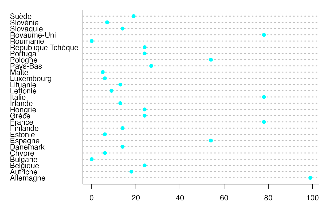
dotchart3(NombreSieges,labels=NameX,pch=19,col="#00FFFF",cex=1.6,cex.axis=.8)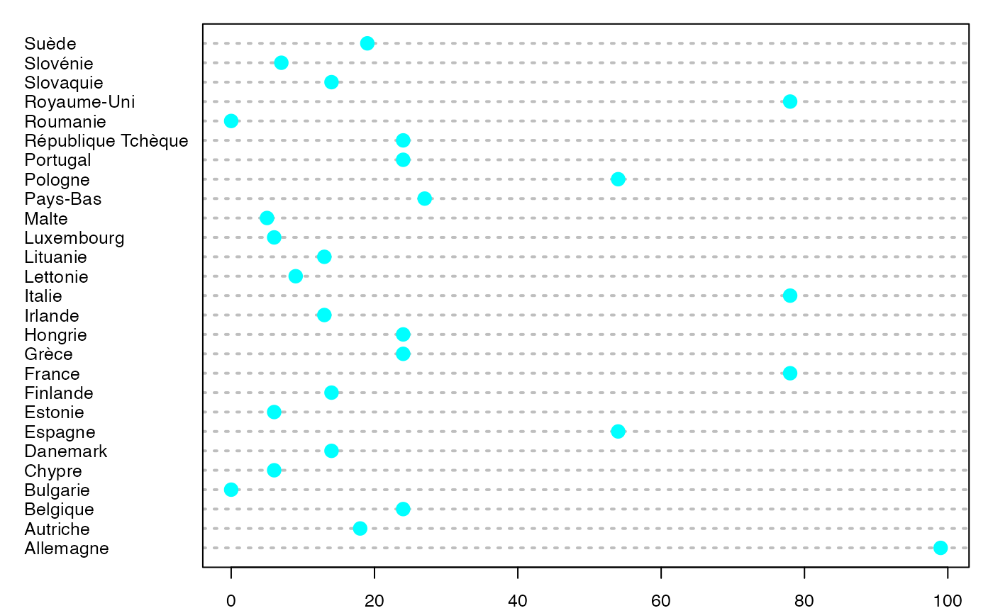
Chemin <- "~/Documents/Recherche/DeBoeck/Graphes/Donnees/"
colmodel="cmyk"
pdf(file = paste(Chemin,"Sieges_pointshoriz_fre.pdf",sep=""),
    width = 8, height = 7, onefile = TRUE, family = "Helvetica",
    title = "Probability or cumulative distribution graphs", paper = "special", colormodel = colmodel)
par(mar = c(2, 2, 1, 1) + 0.1, mgp = c(2, 1, 0))
dotchart3(NombreSieges/sum(NombreSieges),labels=NameX,pch=19,col="#00FFFF",cex=1.6,cex.axis=1.2)
dev.off()
#> agg_png
#>       2
par(mar = c(2, 2, 1, 1) + 0.1, mgp = c(2, 1, 0))
dotchart3(NombreVoix,labels=NameX,pch=19,col="#00FFFF",cex=1.6,cex.axis=1.2)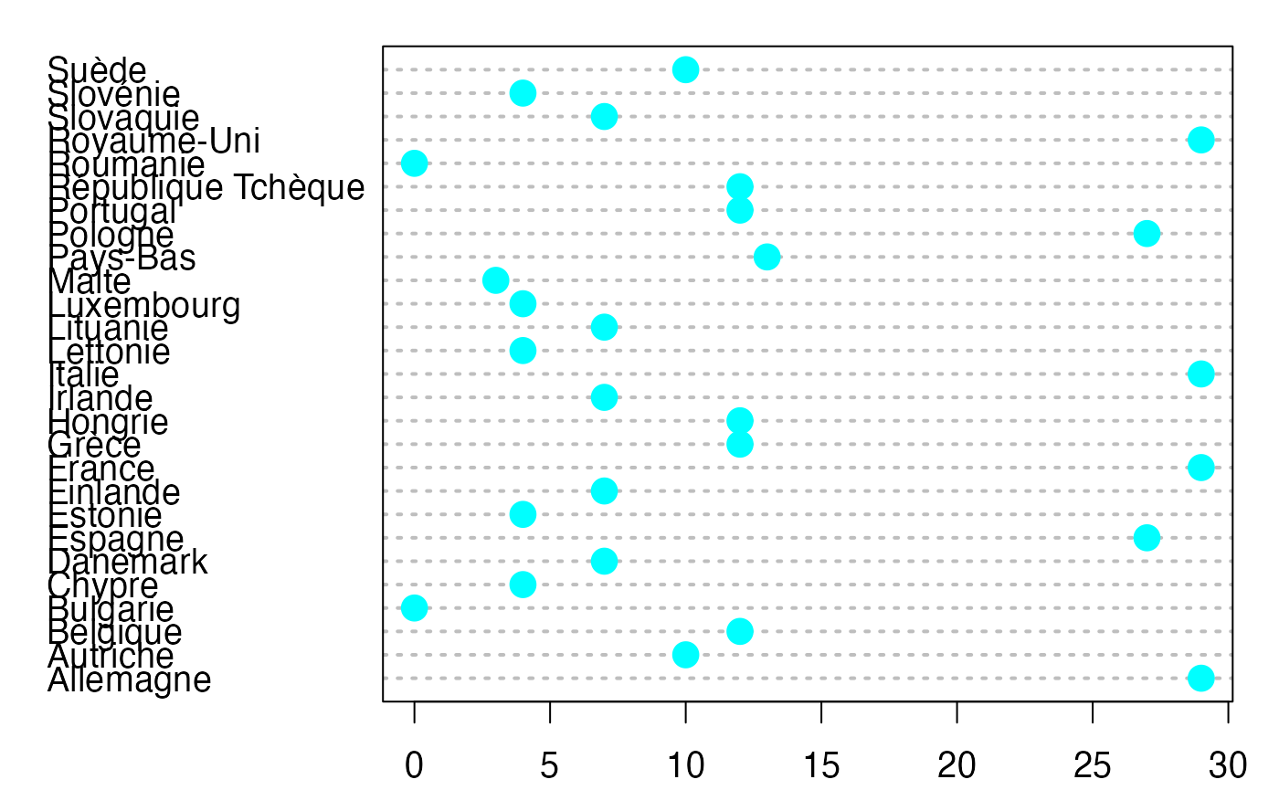
dotchart3(NombreVoix,labels=NameX,pch=19,col="#00FFFF")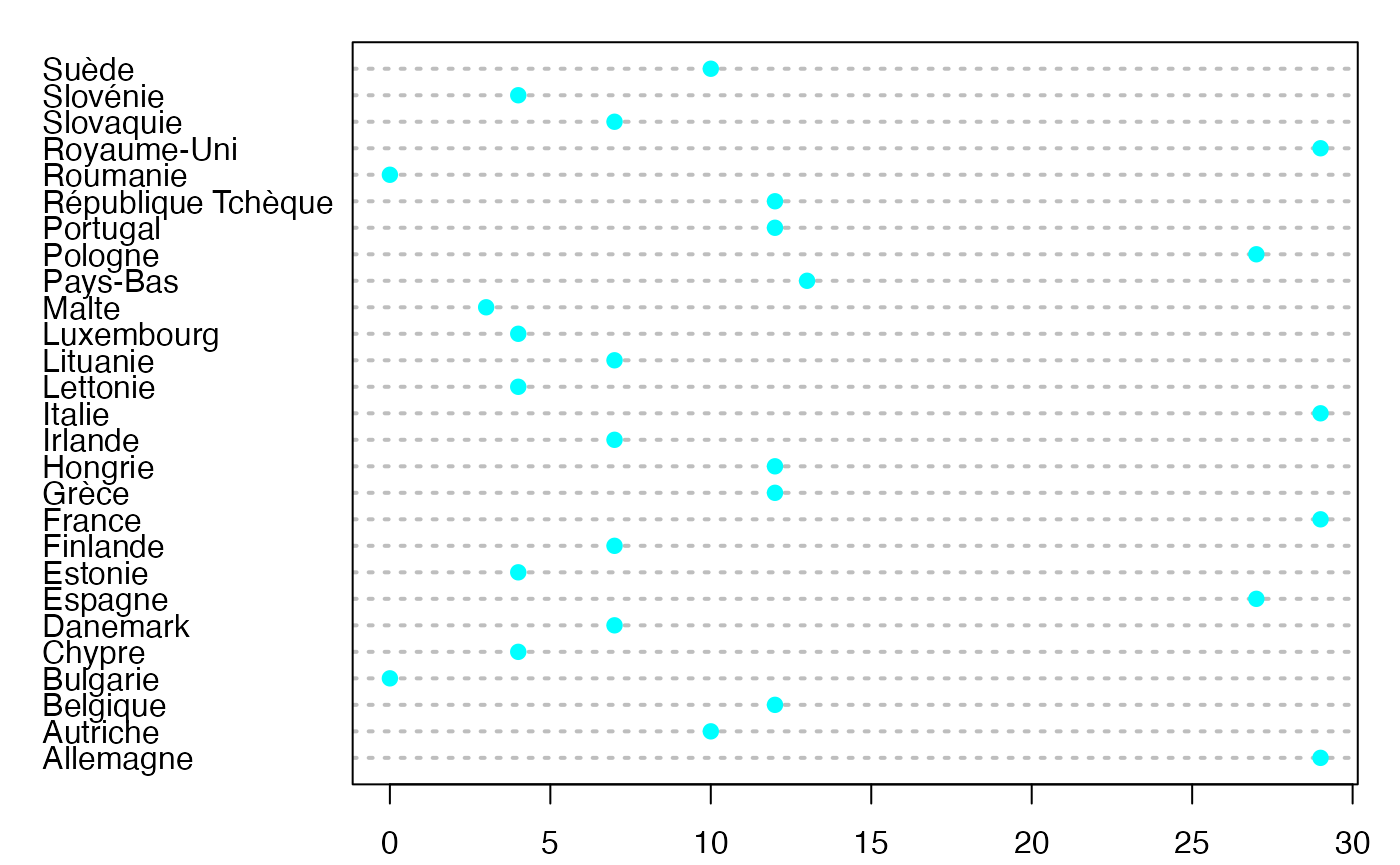
pdf(file = paste(Chemin,"Voix_pointshoriz_fre.pdf",sep=""),
    width = 8, height = 7, onefile = TRUE, family = "Helvetica",
    title = "Probability or cumulative distribution graphs", paper = "special", colormodel = colmodel)
par(mar = c(2, 2, 1, 1) + 0.1, mgp = c(2, 1, 0))
dotchart3(NombreVoix/sum(NombreVoix),labels=NameX,pch=19,col="#00FFFF",cex=1.6,cex.axis=1.2)
dev.off()
#> agg_png
#>       2
par(mar = c(2, 2, 1, 1) + 0.1, mgp = c(2, 1, 0))
dotchart3(NombreAnnees,labels=NameXX,pch=19,col="#00FFFF",cex=1.6,cex.axis=1.2)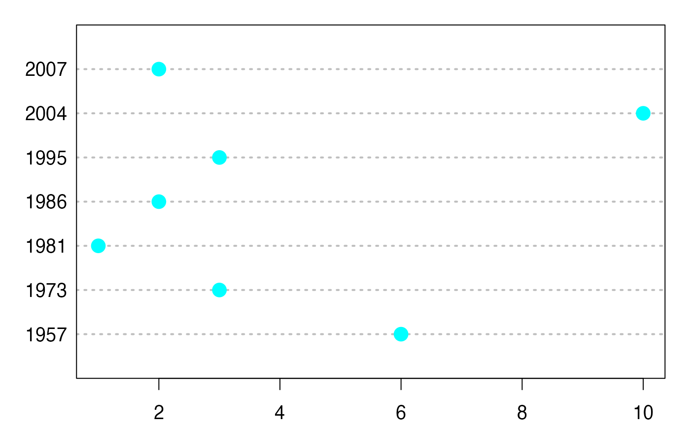
dotchart3(NombreAnnees,labels=NameXX,pch=19,col="#00FFFF")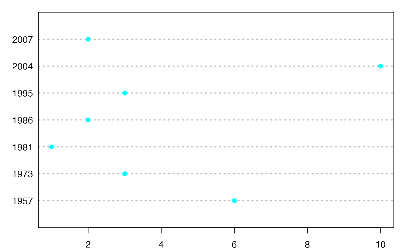
pdf(file = paste(Chemin,"Annees_pointshoriz_fre.pdf",sep=""),
    width = 8, height = 7, onefile = TRUE, family = "Helvetica",
    title = "Probability or cumulative distribution graphs", paper = "special", colormodel = colmodel)
par(mar = c(2, 2, 1, 1) + 0.1, mgp = c(2, 1, 0))
dotchart3(NombreAnnees/sum(NombreAnnees),labels=NameXX,pch=19,col="#00FFFF",cex=1.6,cex.axis=1.2)
dev.off()
#> agg_png
#>       2
NameXbar <- NameX
par(mar = c(9.1, 2, 1, 1) + 0.1, mgp = c(2, 1, 0))
barplot(NombreSieges/sum(NombreSieges),names.arg=NameXbar,col=c("black","#00FFFF","black","#00FFFF"),density = 10,border=c("black","#00FFFF","black","#00FFFF"),cex.axis=1.2,las=3)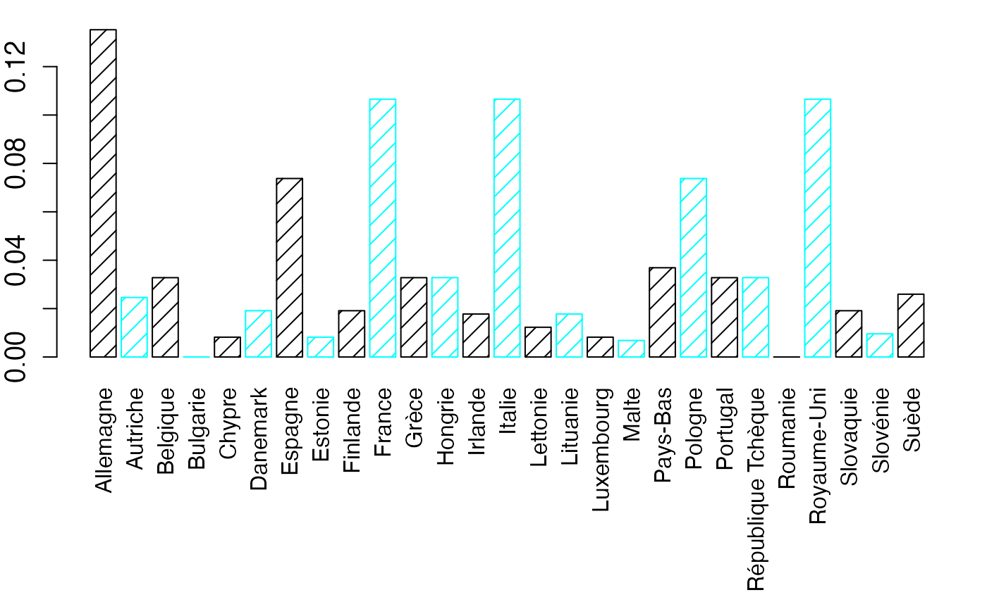
pdf(file = paste(Chemin,"Sieges_barvertibis_fre.pdf",sep=""),
    width = 8, height = 7, onefile = TRUE, family = "Helvetica",
    title = "Probability or cumulative distribution graphs", paper = "special", colormodel = colmodel)
par(mar = c(9.1, 2, 1, 1) + 0.1, mgp = c(2, 1, 0))
barplot(NombreSieges/sum(NombreSieges),names.arg=NameXbar,col=c("black","#00FFFF","black","#00FFFF"),density = 10,border=c("black","#00FFFF","black","#00FFFF"),cex.axis=1.2,las=3)
dev.off()
#> agg_png
#>       2
NameXbar <- NameX
par(mar = c(9.1, 2, 1, 1) + 0.1, mgp = c(2, 1, 0))
barplot(NombreVoix/sum(NombreVoix),names.arg=NameXbar,col=c("black","#00FFFF","black","#00FFFF"),density = 10,border=c("black","#00FFFF","black","#00FFFF"),cex.axis=1.2,las=3)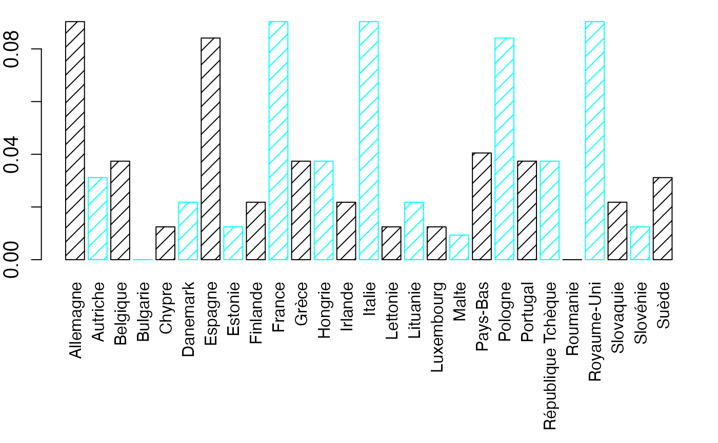
pdf(file = paste(Chemin,"Voix_barvertibis_fre.pdf",sep=""),
    width = 8, height = 7, onefile = TRUE, family = "Helvetica",
    title = "Probability or cumulative distribution graphs", paper = "special", colormodel = colmodel)
par(mar = c(9.1, 2, 1, 1) + 0.1, mgp = c(2, 1, 0))
barplot(NombreVoix/sum(NombreVoix),names.arg=NameXbar,col=c("black","#00FFFF","black","#00FFFF"),density = 10,border=c("black","#00FFFF","black","#00FFFF"),cex.axis=1.2,las=3)
dev.off()
#> agg_png
#>       2
NameXbar <- NameXX
par(mar = c(3.1, 2, 1, 1) + 0.1, mgp = c(2, 1, 0))
barplot(NombreAnnees/sum(NombreAnnees),names.arg=NameXbar,col=c("black","#00FFFF","black","#00FFFF"),density = 10,border=c("black","#00FFFF","black","#00FFFF"),cex.axis=1.2,las=3)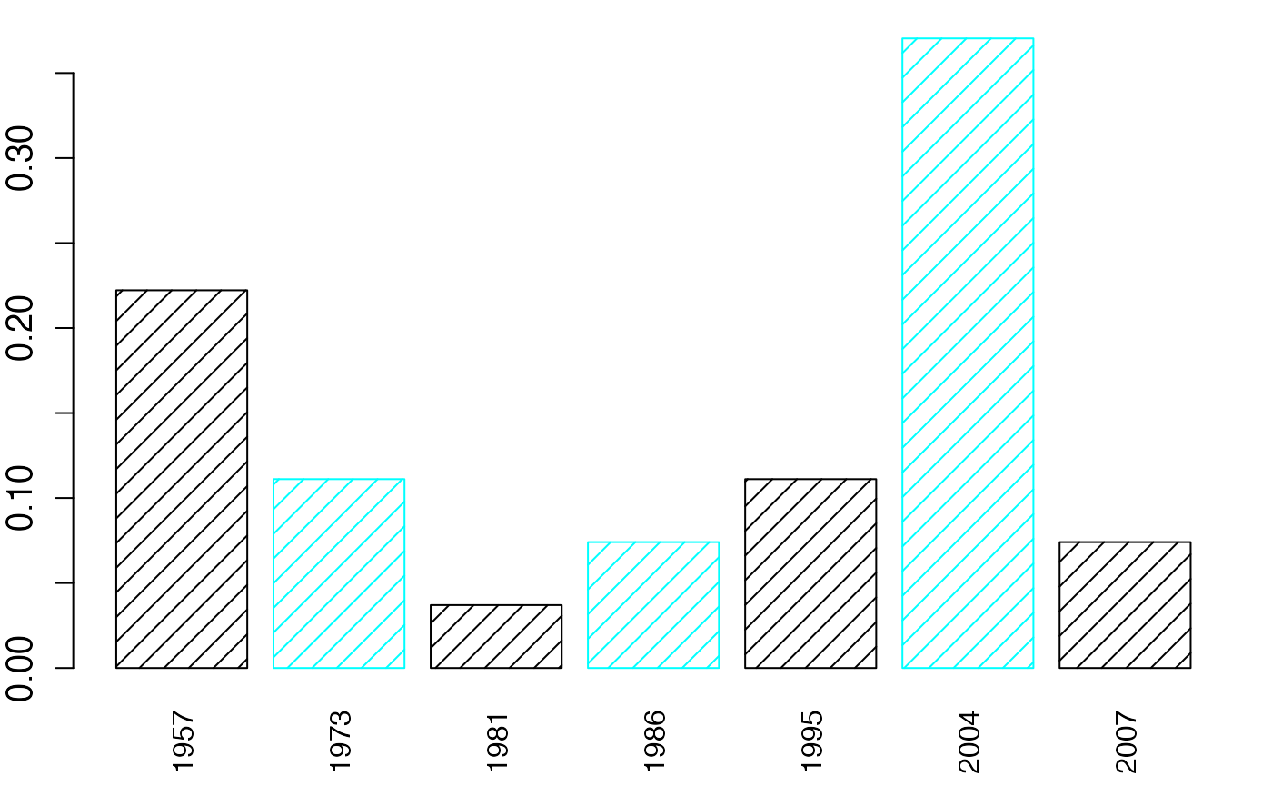
pdf(file = paste(Chemin,"Annees_barvertibis_fre.pdf",sep=""),
    width = 8, height = 7, onefile = TRUE, family = "Helvetica",
    title = "Probability or cumulative distribution graphs", paper = "special", colormodel = colmodel)
par(mar = c(3.1, 2, 1, 1) + 0.1, mgp = c(2, 1, 0))
barplot(NombreAnnees/sum(NombreAnnees),names.arg=NameXbar,col=c("black","#00FFFF","black","#00FFFF"),density = 10,border=c("black","#00FFFF","black","#00FFFF"),cex.axis=1.2,las=3)
dev.off()
#> agg_png
#>       2
NameX[22] <- "République\nTchèque"

par(mar = c(2, 2, 1, 1) + 0.1, mgp = c(2, 1, 0))
pie(NombreSieges,labels=NameX,col=c("black","#00FFFF","black","#00FFFF"),init.angle = 70,density = 10,border=c("black","#00FFFF","black","#00FFFF"),cex=1)#,density = c(4*(4:1))
pdf(file = paste(Chemin,"Sieges_diagcircubis.pdf",sep=""),
    width = 8, height = 7, onefile = TRUE, family = "Helvetica",
    title = "Probability or cumulative distribution graphs", paper = "special", colormodel = colmodel)
par(mar = c(2, 2, 1, 1) + 0.1, mgp = c(2, 1, 0))
pie(NombreSieges,labels=NameX,col=c("black","#00FFFF","black","#00FFFF"),init.angle = 70,density = 10,border=c("black","#00FFFF","black","#00FFFF"),cex=1)#,density = c(4*(4:1))
dev.off()
#> agg_png
#>       2
NameX <- Sieges_Voix$Etats.Membres

par(mar = c(2, 2, 1, 1) + 0.1, mgp = c(2, 1, 0))
pie(NombreVoix,labels=NameX,col=c("black","#00FFFF","black","#00FFFF"),init.angle = 0,density = 10,border=c("black","#00FFFF","black","#00FFFF"),cex=1)#,density = c(4*(4:1))
pdf(file = paste(Chemin,"Voix_diagcircubis.pdf",sep=""),
    width = 8, height = 7, onefile = TRUE, family = "Helvetica",
    title = "Probability or cumulative distribution graphs", paper = "special", colormodel = colmodel)
par(mar = c(2, 2, 1, 1) + 0.1, mgp = c(2, 1, 0))
pie(NombreVoix,labels=NameX,col=c("black","#00FFFF","black","#00FFFF"),init.angle = 0,density = 10,border=c("black","#00FFFF","black","#00FFFF"),cex=1)#,density = c(4*(4:1))
dev.off()
#> agg_png
#>       2
par(mar = c(2, 2, 1, 1) + 0.1, mgp = c(2, 1, 0))
pie(NombreAnnees,labels=NameXX,col=c("black","#00FFFF","black","#00FFFF"),init.angle = 0,density = 10,border=c("black","#00FFFF","black","#00FFFF"),cex=1)#,density = c(4*(4:1))
pdf(file = paste(Chemin,"Annees_diagcircubis.pdf",sep=""),
    width = 8, height = 7, onefile = TRUE, family = "Helvetica",
    title = "Probability or cumulative distribution graphs", paper = "special", colormodel = colmodel)
par(mar = c(2, 2, 1, 1) + 0.1, mgp = c(2, 1, 0))
pie(NombreAnnees,labels=NameXX,col=c("black","#00FFFF","black","#00FFFF"),init.angle = 0,density = 10,border=c("black","#00FFFF","black","#00FFFF"),cex=1)#,density = c(4*(4:1))
dev.off()
#> agg_png
#>       2
Europe Emploi Salariés
Boîte à moustaches
head(europe)
#> [[1]]
#> NULL
#>
#> $Durée
#>  [1] 40.2 41.1 39.1 40.7 41.2 40.4 37.6 39.6 40.2 39.4 39.1 40.7 40.4 39.4 43.4
#> [16] 39.0 40.2 39.9 40.2 41.6 41.3 44.6 38.4 38.9 40.8 40.8 40.6 42.0 42.8 40.5
#> [31] 40.7 39.9 41.8 40.7 48.1
str(europe)
#> List of 2
#>  $      : NULL
#>  $ Durée: num [1:35] 40.2 41.1 39.1 40.7 41.2 40.4 37.6 39.6 40.2 39.4 ...
summary(europe$Durée)
#>    Min. 1st Qu.  Median    Mean 3rd Qu.    Max.
#>   37.60   39.75   40.50   40.72   41.15   48.10
range(europe$Durée)
#> [1] 37.6 48.1
sd(europe$Durée)
#> [1] 1.873984

qts <- quantile(europe$Durée,c(.25,.5,.75),type=6)
ltms <- c(qts[1]-3/2*(qts[3]-qts[1]),qts[3]+3/2*(qts[3]-qts[1]))
lms <- c(min(europe$Durée[europe$Durée>=qts[1]-3/2*(qts[3]-qts[1])]),max(europe$Durée[europe$Durée<=qts[3]+3/2*(qts[3]-qts[1])]))
conf <- qts[2] + c(-1.58, 1.58) * (qts[3]-qts[1])/sqrt(sum(!is.na(europe$Durée)))
extremes <- c(
  europe$Durée[!(europe$Durée>=qts[1]-3/2*(qts[3]-qts[1]))],
  europe$Durée[!(europe$Durée<=qts[3]+3/2*(qts[3]-qts[1]))]
  )


#bltr
oldpar <- par()
par(mar = c(0.2, 3, 0.2, 0.2) + 0.1, mgp = c(2, 1, 0))
bxp(list(stats=t(t(c(lms[1],qts,lms[2]))),n=sum(!is.na(europe$Durée)),conf=matrix(conf,ncol=1)),ylab="Durée (heures)",lwd=2.5,cex.axis=1,cex.lab=1,ylim=range(europe$Durée))
points(1,mean(europe$Durée),pch=2,lwd=2.5,cex=1.25)
points(rep(1,length(extremes)),extremes,pch=8,cex=1.25,lwd=2.5)
Chemin <- "~/Documents/Recherche/DeBoeck/Graphes/Donnees/"
colmodel="cmyk"

pdf(file = paste(Chemin,"boxplot2019v3.pdf",sep=""),
    width = 6, height = 6, onefile = TRUE, family = "Helvetica",
    title = "europeSalaries boxplot", paper = "special")
par(mar = c(0.2, 3, 0.2, 0.2) + 0.1, mgp = c(2, 1, 0))
bxp(list(stats=t(t(c(lms[1],qts,lms[2]))),n=sum(!is.na(europe$Durée)),conf=matrix(conf,ncol=1)),ylab="Durée (heures)",lwd=2.5,cex.axis=1,cex.lab=1,ylim=range(europe$Durée))
points(1,mean(europe$Durée),pch=2,lwd=2.5,cex=1.25)
points(rep(1,length(extremes)),extremes,pch=8,cex=1.25,lwd=2.5)
dev.off()
#> agg_png
#>       2
#suppressWarnings(par(oldpar))
Statistiques descriptives
mean(europe$Durée)
#> [1] 40.72286
quantile(europe$Durée,probs=c(.25,.5,.75),type=6)
#>  25%  50%  75%
#> 39.6 40.5 41.2
range(europe$Durée)
#> [1] 37.6 48.1

diff(quantile(europe$Durée,probs=c(.25,.75),type=6))
#> 75%
#> 1.6
diff(range(europe$Durée))
#> [1] 10.5
1/length(europe$Durée)*sum((europe$Durée-mean(europe$Durée))^2)
#> [1] 3.411478
sqrt(1/length(europe$Durée)*sum((europe$Durée-mean(europe$Durée))^2))
#> [1] 1.847019

sqrt(1/length(europe$Durée)*sum((europe$Durée-mean(europe$Durée))^2))/mean(europe$Durée)*100
#> [1] 4.535582
mean(sort(abs(europe$Durée-mean(sort(europe$Durée)[c(14)])))[c(14)])
#> [1] 0.5


1/length(europe$Durée)*sum((europe$Durée-mean(europe$Durée))^3)/((1/length(europe$Durée)*sum((europe$Durée-mean(europe$Durée))^2))^(3/2))
#> [1] 1.912403
(1/length(europe$Durée)*sum((europe$Durée-mean(europe$Durée))^3)/((1/length(europe$Durée)*sum((europe$Durée-mean(europe$Durée))^2))^(3/2)))^2
#> [1] 3.657286

1/length(europe$Durée)*sum((europe$Durée-mean(europe$Durée))^4)/((1/length(europe$Durée)*sum((europe$Durée-mean(europe$Durée))^2))^(4/2))
#> [1] 8.419112
1/length(europe$Durée)*sum((europe$Durée-mean(europe$Durée))^4)/((1/length(europe$Durée)*sum((europe$Durée-mean(europe$Durée))^2))^(4/2))-3
#> [1] 5.419112
Europe Emploi Non-Salariés
Boîte à moustaches
head(europe)
#> [[1]]
#> NULL
#>
#> $Durée
#>  [1] 47.6 51.2 52.5 43.0 44.9 44.6 46.3 47.0 43.2 46.4 50.1 50.4 41.5 49.4 48.5
#> [16] 46.0 41.5 40.6 46.9 45.3 47.4 48.3 45.0 47.9 45.7 47.6 38.9 45.2 51.2 45.1
#> [31] 45.7 47.9 49.4 45.9 49.6
str(europe)
#> List of 2
#>  $      : NULL
#>  $ Durée: num [1:35] 47.6 51.2 52.5 43 44.9 44.6 46.3 47 43.2 46.4 ...
summary(europe$Durée)
#>    Min. 1st Qu.  Median    Mean 3rd Qu.    Max.
#>   38.90   45.05   46.40   46.51   48.40   52.50
range(europe$Durée)
#> [1] 38.9 52.5
sd(europe$Durée)
#> [1] 3.118912

qts <- quantile(europe$Durée,c(.25,.5,.75),type=6)
ltms <- c(qts[1]-3/2*(qts[3]-qts[1]),qts[3]+3/2*(qts[3]-qts[1]))
lms <- c(min(europe$Durée[europe$Durée>=qts[1]-3/2*(qts[3]-qts[1])]),max(europe$Durée[europe$Durée<=qts[3]+3/2*(qts[3]-qts[1])]))
conf <- qts[2] + c(-1.58, 1.58) * (qts[3]-qts[1])/sqrt(sum(!is.na(europe$Durée)))
extremes <- c(
  europe$Durée[!(europe$Durée>=qts[1]-3/2*(qts[3]-qts[1]))],
  europe$Durée[!(europe$Durée<=qts[3]+3/2*(qts[3]-qts[1]))]
  )


#bltr
oldpar <- par()
par(mar = c(0.2, 3, 0.2, 0.2) + 0.1, mgp = c(2, 1, 0))
bxp(list(stats=t(t(c(lms[1],qts,lms[2]))),n=sum(!is.na(europe$Durée)),conf=matrix(conf,ncol=1)),ylab="Durée (heures)",lwd=2.5,cex.axis=1,cex.lab=1,ylim=range(europe$Durée))
points(1,mean(europe$Durée),pch=2,lwd=2.5,cex=1.25)
points(rep(1,length(extremes)),extremes,pch=8,cex=1.25,lwd=2.5)
Chemin <- "~/Documents/Recherche/DeBoeck/Graphes/Donnees/"
colmodel="cmyk"
pdf(file = paste(Chemin,"boxplot2019v3_app2.pdf",sep=""),
    width = 6, height = 6, onefile = TRUE, family = "Helvetica",
    title = "europeSalaries boxplot", paper = "special")
par(mar = c(0.2, 3, 0.2, 0.2) + 0.1, mgp = c(2, 1, 0))
bxp(list(stats=t(t(c(lms[1],qts,lms[2]))),n=sum(!is.na(europe$Durée)),conf=matrix(conf,ncol=1)),ylab="Durée (heures)",lwd=2.5,cex.axis=1,cex.lab=1,ylim=range(europe$Durée))
points(1,mean(europe$Durée),pch=2,lwd=2.5,cex=1.25)
points(rep(1,length(extremes)),extremes,pch=8,cex=1.25,lwd=2.5)
dev.off()
#> agg_png
#>       2
#suppressWarnings(par(oldpar))
Statistiques descriptives
mean(europe$Durée)
#> [1] 46.50571
quantile(europe$Durée,probs=c(.25,.5,.75),type=6)
#>  25%  50%  75%
#> 45.0 46.4 48.5
range(europe$Durée)
#> [1] 38.9 52.5

diff(quantile(europe$Durée,probs=c(.25,.75),type=6))
#> 75%
#> 3.5
diff(range(europe$Durée))
#> [1] 13.6
1/length(europe$Durée)*sum((europe$Durée-mean(europe$Durée))^2)
#> [1] 9.449682
sqrt(1/length(europe$Durée)*sum((europe$Durée-mean(europe$Durée))^2))
#> [1] 3.074033

sqrt(1/length(europe$Durée)*sum((europe$Durée-mean(europe$Durée))^2))/mean(europe$Durée)*100
#> [1] 6.610012
mean(sort(abs(europe$Durée-mean(sort(europe$Durée)[c(14)])))[c(14)])
#> [1] 1.3


1/length(europe$Durée)*sum((europe$Durée-mean(europe$Durée))^3)/((1/length(europe$Durée)*sum((europe$Durée-mean(europe$Durée))^2))^(3/2))
#> [1] -0.3640395
(1/length(europe$Durée)*sum((europe$Durée-mean(europe$Durée))^3)/((1/length(europe$Durée)*sum((europe$Durée-mean(europe$Durée))^2))^(3/2)))^2
#> [1] 0.1325248

1/length(europe$Durée)*sum((europe$Durée-mean(europe$Durée))^4)/((1/length(europe$Durée)*sum((europe$Durée-mean(europe$Durée))^2))^(4/2))
#> [1] 2.896399
1/length(europe$Durée)*sum((europe$Durée-mean(europe$Durée))^4)/((1/length(europe$Durée)*sum((europe$Durée-mean(europe$Durée))^2))^(4/2))-3
#> [1] -0.1036008
Europe Emploi Partiel_Ens
data(Europe)
europe <- vector("list",1)
europe$Durée <- Europe$Partiel_Ens

head(europe)
#> [[1]]
#> NULL
#>
#> $Durée
#>  [1] 27.2 27.2 24.9  1.9 10.2  4.8 24.2 14.5 11.3 15.5 17.5  9.1  4.4 19.7 21.5
#> [16] 18.7  8.4  6.4 17.0  4.1 12.2  4.5 25.8 50.2  6.1  8.1  6.1 24.4  9.7  4.5
#> [31]  8.4 22.5 38.0  6.3  9.9
str(europe)
#> List of 2
#>  $      : NULL
#>  $ Durée: num [1:35] 27.2 27.2 24.9 1.9 10.2 4.8 24.2 14.5 11.3 15.5 ...
summary(europe)
#>       Length Class  Mode
#>        0     -none- NULL
#> Durée 35     -none- numeric
range(europe$Durée)
#> [1]  1.9 50.2
sd(europe$Durée)
#> [1] 10.71283


rangePartiel_Ens <-
cbind(range(Europe$Partiel_Ens),
range(Europe$Partiel_H),
range(Europe$Partiel_F))

ylimits = c(min(rangePartiel_Ens[1,]),
max(rangePartiel_Ens[2,]))
Boîte à moustaches
qts <- quantile(europe$Durée,c(.25,.5,.75),type=6)
ltms <- c(qts[1]-3/2*(qts[3]-qts[1]),qts[3]+3/2*(qts[3]-qts[1]))
lms <- c(min(europe$Durée[europe$Durée>=qts[1]-3/2*(qts[3]-qts[1])]),max(europe$Durée[europe$Durée<=qts[3]+3/2*(qts[3]-qts[1])]))
conf <- qts[2] + c(-1.58, 1.58) * (qts[3]-qts[1])/sqrt(sum(!is.na(europe$Durée)))


#bltr
oldpar <- par()
par(mar = c(0.2, 3, 0.2, 0.2) + 0.1, mgp = c(2, 1, 0))
bxp(list(stats=t(t(c(lms[1],qts,lms[2]))),n=sum(!is.na(europe$Durée)),conf=matrix(conf,ncol=1)),ylab="% emploi total",lwd=2.5,cex.axis=1,cex.lab=1,ylim=range(europe$Durée))
points(1,mean(europe$Durée),pch=2,lwd=2.5,cex=1.25)
points(1,
  c(
  europe$Durée[!(europe$Durée>=qts[1]-3/2*(qts[3]-qts[1]))],
  europe$Durée[!(europe$Durée<=qts[3]+3/2*(qts[3]-qts[1]))]
  ),pch=8,cex=1.25,lwd=2.5
  )
Chemin <- "~/Documents/Recherche/DeBoeck/Graphes/Donnees/"
colmodel="cmyk"
pdf(file = paste(Chemin,"boxplotPartiel_Ens.pdf",sep=""),
    width = 6, height = 6, onefile = TRUE, family = "Helvetica",
    title = "Europe boxplot", paper = "special")
par(mar = c(0.2, 3, 0.2, 0.2) + 0.1, mgp = c(2, 1, 0))
bxp(list(stats=t(t(c(lms[1],qts,lms[2]))),n=sum(!is.na(europe$Durée)),conf=matrix(conf,ncol=1)),ylab="% emploi total",lwd=2.5,cex.axis=1,cex.lab=1,ylim=range(europe$Durée))
points(1,mean(europe$Durée),pch=2,lwd=2.5,cex=1.25)
points(1,
  c(
  europe$Durée[!(europe$Durée>=qts[1]-3/2*(qts[3]-qts[1]))],
  europe$Durée[!(europe$Durée<=qts[3]+3/2*(qts[3]-qts[1]))]
  ),pch=8,cex=1.25,lwd=2.5
  )
dev.off()
#> agg_png
#>       2

pdf(file = paste(Chemin,"boxplotPartiel_Ens_same_scale.pdf",sep=""),
    width = 6, height = 6, onefile = TRUE, family = "Helvetica",
    title = "Europe boxplot", paper = "special")
par(mar = c(0.2, 3, 0.2, 0.2) + 0.1, mgp = c(2, 1, 0))
bxp(list(stats=t(t(c(lms[1],qts,lms[2]))),n=sum(!is.na(europe$Durée)),conf=matrix(conf,ncol=1)),ylab="% emploi total",lwd=2.5,cex.axis=1,cex.lab=1,ylim=ylimits)
points(1,mean(europe$Durée),pch=2,lwd=2.5,cex=1.25)
points(1,
  c(
  europe$Durée[!(europe$Durée>=qts[1]-3/2*(qts[3]-qts[1]))],
  europe$Durée[!(europe$Durée<=qts[3]+3/2*(qts[3]-qts[1]))]
  ),pch=8,cex=1.25,lwd=2.5
  )
dev.off()
#> agg_png
#>       2
Statistiques descriptives
mean(europe$Durée)
#> [1] 15.00571
quantile(europe$Durée,probs=c(.25,.5,.75),type=6)
#>  25%  50%  75%
#>  6.3 11.3 22.5
range(europe$Durée)
#> [1]  1.9 50.2

diff(quantile(europe$Durée,probs=c(.25,.75),type=6))
#>  75%
#> 16.2
diff(range(europe$Durée))
#> [1] 48.3
1/length(europe$Durée)*sum((europe$Durée-mean(europe$Durée))^2)
#> [1] 111.4857
sqrt(1/length(europe$Durée)*sum((europe$Durée-mean(europe$Durée))^2))
#> [1] 10.55868

sqrt(1/length(europe$Durée)*sum((europe$Durée-mean(europe$Durée))^2))/mean(europe$Durée)*100
#> [1] 70.36438
mean(sort(abs(europe$Durée-mean(sort(europe$Durée)[c(14)])))[c(14)])
#> [1] 4.3


1/length(europe$Durée)*sum((europe$Durée-mean(europe$Durée))^3)/((1/length(europe$Durée)*sum((europe$Durée-mean(europe$Durée))^2))^(3/2))
#> [1] 1.254157
(1/length(europe$Durée)*sum((europe$Durée-mean(europe$Durée))^3)/((1/length(europe$Durée)*sum((europe$Durée-mean(europe$Durée))^2))^(3/2)))^2
#> [1] 1.57291

1/length(europe$Durée)*sum((europe$Durée-mean(europe$Durée))^4)/((1/length(europe$Durée)*sum((europe$Durée-mean(europe$Durée))^2))^(4/2))
#> [1] 4.658759
1/length(europe$Durée)*sum((europe$Durée-mean(europe$Durée))^4)/((1/length(europe$Durée)*sum((europe$Durée-mean(europe$Durée))^2))^(4/2))-3
#> [1] 1.658759
Europe Emploi Partiel_H
data(Europe)

europe <- vector("list",1)
europe$Durée <- Europe$Partiel_H

head(europe)
#> [[1]]
#> NULL
#>
#> $Durée
#>  [1]  9.9  9.5 10.5  1.7  6.3  3.1 15.3  6.8  7.1 10.1  7.5  5.9  2.5 10.1 10.3
#> [16]  8.2  5.8  4.7  5.6  4.1  5.9  4.7 15.2 27.9  3.5  5.4  6.0 10.8  8.9  2.9
#> [31]  4.8 13.4 17.1  2.8  6.6
str(europe)
#> List of 2
#>  $      : NULL
#>  $ Durée: num [1:35] 9.9 9.5 10.5 1.7 6.3 3.1 15.3 6.8 7.1 10.1 ...
summary(europe)
#>       Length Class  Mode
#>        0     -none- NULL
#> Durée 35     -none- numeric
range(europe$Durée)
#> [1]  1.7 27.9
sd(europe$Durée)
#> [1] 5.144977
Boîte à moustaches
qts <- quantile(europe$Durée,c(.25,.5,.75),type=6)
ltms <- c(qts[1]-3/2*(qts[3]-qts[1]),qts[3]+3/2*(qts[3]-qts[1]))
lms <- c(min(europe$Durée[europe$Durée>=qts[1]-3/2*(qts[3]-qts[1])]),max(europe$Durée[europe$Durée<=qts[3]+3/2*(qts[3]-qts[1])]))
conf <- qts[2] + c(-1.58, 1.58) * (qts[3]-qts[1])/sqrt(sum(!is.na(europe$Durée)))

#bltr
oldpar <- par()
par(mar = c(0.2, 3, 0.2, 0.2) + 0.1, mgp = c(2, 1, 0))
bxp(list(stats=t(t(c(lms[1],qts,lms[2]))),n=sum(!is.na(europe$Durée)),conf=matrix(conf,ncol=1)),ylab="% emploi total",lwd=2.5,cex.axis=1,cex.lab=1,ylim=range(europe$Durée))
points(1,mean(europe$Durée),pch=2,lwd=2.5,cex=1.25)
points(1,
  c(
  europe$Durée[!(europe$Durée>=qts[1]-3/2*(qts[3]-qts[1]))],
  europe$Durée[!(europe$Durée<=qts[3]+3/2*(qts[3]-qts[1]))]
  ),pch=8,cex=1.25,lwd=2.5
  )
Chemin <- "~/Documents/Recherche/DeBoeck/Graphes/Donnees/"
colmodel="cmyk"
pdf(file = paste(Chemin,"boxplotPartiel_H.pdf",sep=""),
    width = 6, height = 6, onefile = TRUE, family = "Helvetica",
    title = "Europe boxplot", paper = "special")
par(mar = c(0.2, 3, 0.2, 0.2) + 0.1, mgp = c(2, 1, 0))
bxp(list(stats=t(t(c(lms[1],qts,lms[2]))),n=sum(!is.na(europe$Durée)),conf=matrix(conf,ncol=1)),ylab="% emploi total",lwd=2.5,cex.axis=1,cex.lab=1,ylim=range(europe$Durée))
points(1,mean(europe$Durée),pch=2,lwd=2.5,cex=1.25)
points(1,
  c(
  europe$Durée[!(europe$Durée>=qts[1]-3/2*(qts[3]-qts[1]))],
  europe$Durée[!(europe$Durée<=qts[3]+3/2*(qts[3]-qts[1]))]
  ),pch=8,cex=1.25,lwd=2.5
  )
dev.off()
#> agg_png
#>       2

pdf(file = paste(Chemin,"boxplotPartiel_H_same_scale.pdf",sep=""),
    width = 6, height = 6, onefile = TRUE, family = "Helvetica",
    title = "Europe boxplot", paper = "special")
par(mar = c(0.2, 3, 0.2, 0.2) + 0.1, mgp = c(2, 1, 0))
bxp(list(stats=t(t(c(lms[1],qts,lms[2]))),n=sum(!is.na(europe$Durée)),conf=matrix(conf,ncol=1)),ylab="% emploi total",lwd=2.5,cex.axis=1,cex.lab=1,ylim=ylimits)
points(1,mean(europe$Durée),pch=2,lwd=2.5,cex=1.25)
points(1,
  c(
  europe$Durée[!(europe$Durée>=qts[1]-3/2*(qts[3]-qts[1]))],
  europe$Durée[!(europe$Durée<=qts[3]+3/2*(qts[3]-qts[1]))]
  ),pch=8,cex=1.25,lwd=2.5
  )
dev.off()
#> agg_png
#>       2
Statistiques descriptives
mean(europe$Durée)
#> [1] 8.025714
quantile(europe$Durée,probs=c(.25,.5,.75),type=6)
#>  25%  50%  75%
#>  4.7  6.6 10.1
range(europe$Durée)
#> [1]  1.7 27.9

diff(quantile(europe$Durée,probs=c(.25,.75),type=6))
#> 75%
#> 5.4
diff(range(europe$Durée))
#> [1] 26.2
1/length(europe$Durée)*sum((europe$Durée-mean(europe$Durée))^2)
#> [1] 25.71448
sqrt(1/length(europe$Durée)*sum((europe$Durée-mean(europe$Durée))^2))
#> [1] 5.070945

sqrt(1/length(europe$Durée)*sum((europe$Durée-mean(europe$Durée))^2))/mean(europe$Durée)*100
#> [1] 63.18372
mean(sort(abs(europe$Durée-mean(sort(europe$Durée)[c(14)])))[c(14)])
#> [1] 1.6


1/length(europe$Durée)*sum((europe$Durée-mean(europe$Durée))^3)/((1/length(europe$Durée)*sum((europe$Durée-mean(europe$Durée))^2))^(3/2))
#> [1] 1.845463
(1/length(europe$Durée)*sum((europe$Durée-mean(europe$Durée))^3)/((1/length(europe$Durée)*sum((europe$Durée-mean(europe$Durée))^2))^(3/2)))^2
#> [1] 3.405734

1/length(europe$Durée)*sum((europe$Durée-mean(europe$Durée))^4)/((1/length(europe$Durée)*sum((europe$Durée-mean(europe$Durée))^2))^(4/2))
#> [1] 7.561845
1/length(europe$Durée)*sum((europe$Durée-mean(europe$Durée))^4)/((1/length(europe$Durée)*sum((europe$Durée-mean(europe$Durée))^2))^(4/2))-3
#> [1] 4.561845
Europe Emploi Partiel_F
data(Europe)

europe <- vector("list",1)
europe$Durée <- Europe$Partiel_F

head(europe)
#> [[1]]
#> NULL
#>
#> $Durée
#>  [1] 46.7 47.1 41.0  2.1 14.6  6.7 33.9 23.7 15.9 21.3 28.0 13.5  6.8 30.6 34.1
#> [16] 32.9 10.9  8.0 30.4  4.3 21.4  4.1 37.7 75.2  9.3 10.9  6.2 39.4 10.6  6.5
#> [31] 12.7 32.5 61.7 10.6 17.0
str(europe)
#> List of 2
#>  $      : NULL
#>  $ Durée: num [1:35] 46.7 47.1 41 2.1 14.6 6.7 33.9 23.7 15.9 21.3 ...
summary(europe)
#>       Length Class  Mode
#>        0     -none- NULL
#> Durée 35     -none- numeric
range(europe$Durée)
#> [1]  2.1 75.2
sd(europe$Durée)
#> [1] 17.43912
Boîte à moustaches
qts <- quantile(europe$Durée,c(.25,.5,.75),type=6)
ltms <- c(qts[1]-3/2*(qts[3]-qts[1]),qts[3]+3/2*(qts[3]-qts[1]))
lms <- c(min(europe$Durée[europe$Durée>=qts[1]-3/2*(qts[3]-qts[1])]),max(europe$Durée[europe$Durée<=qts[3]+3/2*(qts[3]-qts[1])]))
conf <- qts[2] + c(-1.58, 1.58) * (qts[3]-qts[1])/sqrt(sum(!is.na(europe$Durée)))


#bltr
oldpar <- par()
par(mar = c(0.2, 3, 0.2, 0.2) + 0.1, mgp = c(2, 1, 0))
bxp(list(stats=t(t(c(lms[1],qts,lms[2]))),n=sum(!is.na(europe$Durée)),conf=matrix(conf,ncol=1)),ylab="% emploi total",lwd=2.5,cex.axis=1,cex.lab=1,ylim=range(europe$Durée))
points(1,mean(europe$Durée),pch=2,lwd=2.5,cex=1.25)
points(1,
  c(
  europe$Durée[!(europe$Durée>=qts[1]-3/2*(qts[3]-qts[1]))],
  europe$Durée[!(europe$Durée<=qts[3]+3/2*(qts[3]-qts[1]))]
  ),pch=8,cex=1.25,lwd=2.5
  )
Chemin <- "~/Documents/Recherche/DeBoeck/Graphes/Donnees/"
colmodel="cmyk"
pdf(file = paste(Chemin,"boxplotPartiel_F.pdf",sep=""),
    width = 6, height = 6, onefile = TRUE, family = "Helvetica",
    title = "Europe boxplot", paper = "special")
par(mar = c(0.2, 3, 0.2, 0.2) + 0.1, mgp = c(2, 1, 0))
bxp(list(stats=t(t(c(lms[1],qts,lms[2]))),n=sum(!is.na(europe$Durée)),conf=matrix(conf,ncol=1)),ylab="% emploi total",lwd=2.5,cex.axis=1,cex.lab=1,ylim=range(europe$Durée))
points(1,mean(europe$Durée),pch=2,lwd=2.5,cex=1.25)
points(1,
  c(
  europe$Durée[!(europe$Durée>=qts[1]-3/2*(qts[3]-qts[1]))],
  europe$Durée[!(europe$Durée<=qts[3]+3/2*(qts[3]-qts[1]))]
  ),pch=8,cex=1.25,lwd=2.5
  )
dev.off()
#> agg_png
#>       2

pdf(file = paste(Chemin,"boxplotPartiel_F_same_scale.pdf",sep=""),
    width = 6, height = 6, onefile = TRUE, family = "Helvetica",
    title = "Europe boxplot", paper = "special")
par(mar = c(0.2, 3, 0.2, 0.2) + 0.1, mgp = c(2, 1, 0))
bxp(list(stats=t(t(c(lms[1],qts,lms[2]))),n=sum(!is.na(europe$Durée)),conf=matrix(conf,ncol=1)),ylab="% emploi total",lwd=2.5,cex.axis=1,cex.lab=1,ylim=ylimits)
points(1,mean(europe$Durée),pch=2,lwd=2.5,cex=1.25)
points(1,
  c(
  europe$Durée[!(europe$Durée>=qts[1]-3/2*(qts[3]-qts[1]))],
  europe$Durée[!(europe$Durée<=qts[3]+3/2*(qts[3]-qts[1]))]
  ),pch=8,cex=1.25,lwd=2.5
  )
dev.off()
#> agg_png
#>       2
Statistiques descriptives
mean(europe$Durée)
#> [1] 23.09429
quantile(europe$Durée,probs=c(.25,.5,.75),type=6)
#>  25%  50%  75%
#>  9.3 17.0 33.9
range(europe$Durée)
#> [1]  2.1 75.2

diff(quantile(europe$Durée,probs=c(.25,.75),type=6))
#>  75%
#> 24.6
diff(range(europe$Durée))
#> [1] 73.1
1/length(europe$Durée)*sum((europe$Durée-mean(europe$Durée))^2)
#> [1] 295.4337
sqrt(1/length(europe$Durée)*sum((europe$Durée-mean(europe$Durée))^2))
#> [1] 17.18818

sqrt(1/length(europe$Durée)*sum((europe$Durée-mean(europe$Durée))^2))/mean(europe$Durée)*100
#> [1] 74.42614
mean(sort(abs(europe$Durée-mean(sort(europe$Durée)[c(14)])))[c(14)])
#> [1] 6.2


1/length(europe$Durée)*sum((europe$Durée-mean(europe$Durée))^3)/((1/length(europe$Durée)*sum((europe$Durée-mean(europe$Durée))^2))^(3/2))
#> [1] 1.051022
(1/length(europe$Durée)*sum((europe$Durée-mean(europe$Durée))^3)/((1/length(europe$Durée)*sum((europe$Durée-mean(europe$Durée))^2))^(3/2)))^2
#> [1] 1.104648

1/length(europe$Durée)*sum((europe$Durée-mean(europe$Durée))^4)/((1/length(europe$Durée)*sum((europe$Durée-mean(europe$Durée))^2))^(4/2))
#> [1] 3.753343
1/length(europe$Durée)*sum((europe$Durée-mean(europe$Durée))^4)/((1/length(europe$Durée)*sum((europe$Durée-mean(europe$Durée))^2))^(4/2))-3
#> [1] 0.753343
Partiel Ensemble
data(Europe)

var1<- Europe$Partiel_Ens
varN <- "_Ens"

xi <- unique(sort(var1))
ni <- as.vector(table(var1))

data2 <- cbind(xi,ni)
Diagramme en bâtons des effectifs
oldpar <- par()
par(mar = c(2, 2, 1, 1) + 0.1, mgp=c(2,1,0))
plot(xi,ni,type='h',xlab="",ylab="",lwd=2,ylim=c(0,max(ni))) #,xaxt="n"
#axis(1, at = 1:6, labels = c(1:5,6))
#axis(1, at = 1:6, labels = c(1:5,"6 et plus"))
#suppressWarnings(par(oldpar))
Chemin <- "~/Documents/Recherche/DeBoeck/Graphes/Donnees/"
colmodel="cmyk"
pdf(file = paste(Chemin,"batoneffnew",varN,".pdf",sep=""),
    width = 8, height = 7, onefile = TRUE, family = "Helvetica",
    title = "Diagramme en bâtons des effectifs", paper = "special", colormodel = colmodel)
par(mar = c(2, 2, 1, 1) + 0.1, mgp = c(2, 1, 0))
plot(xi,ni,type='h',xlab="",ylab="",lwd=2,ylim=c(0,max(ni))) #,xaxt="n"
dev.off()
#> agg_png
#>       2
Diagramme en bâtons des fréquences
oldpar <- par()
par(mar = c(2, 2, 1, 1) + 0.1, mgp=c(2,1,0))
plot(xi,ni/sum(ni),type='h',xlab="",ylab="",lwd=2,ylim=c(0,max(ni/sum(ni))))   #,xaxt="n"
#suppressWarnings(par(oldpar))
pdf(file = paste(Chemin,"batonfrenew",varN,".pdf",sep=""),
    width = 8, height = 7, onefile = TRUE, family = "Helvetica",
    title = "Diagramme en bâtons des fréquences", paper = "special", colormodel = colmodel)
par(mar = c(2, 2, 1, 1) + 0.1, mgp = c(2, 1, 0))
plot(xi,ni/sum(ni),type='h',xlab="",ylab="",lwd=2,ylim=c(0,max(ni/sum(ni))))   #,xaxt="n"
dev.off()
#> agg_png
#>       2
Diagramme en bâtons des effectifs et polygone des effectifs
oldpar <- par()
par(mar = c(2, 2, 1, 1) + 0.1, mgp=c(2,1,0))
plot(xi,ni,type='h',xlab="",ylab="",lwd=2,ylim=c(0,max(ni))) #,xaxt="n"
segments(xi[-length(xi)],ni[-length(xi)],xi[-1],ni[-1],lwd=2,col="#00FFFF")
#suppressWarnings(par(oldpar))
pdf(file = paste(Chemin,"polyeffnew",varN,".pdf",sep=""),
    width = 8, height = 7, onefile = TRUE, family = "Helvetica",
    title = "Diagramme en bâtons des effectifs et polygone des effectifs", paper = "special", colormodel = colmodel)
par(mar = c(2, 2, 1, 1) + 0.1, mgp = c(2, 1, 0))
plot(xi,ni,type='h',xlab="",ylab="",lwd=2,ylim=c(0,max(ni))) #,xaxt="n"
segments(xi[-length(xi)],ni[-length(xi)],xi[-1],ni[-1],lwd=2,col="#00FFFF")
dev.off()
#> agg_png
#>       2
Diagramme en bâtons des fréquences et polygone des fréquences
oldpar <- par()
par(mar = c(2, 2, 1, 1) + 0.1, mgp=c(2,1,0))
plot(xi,ni/sum(ni),type='h',xlab="",ylab="",lwd=2,ylim=c(0,max(ni/sum(ni))))
segments(xi[-length(xi)],ni[-length(xi)]/sum(ni),xi[-1],ni[-1]/sum(ni),lwd=2,col="#00FFFF")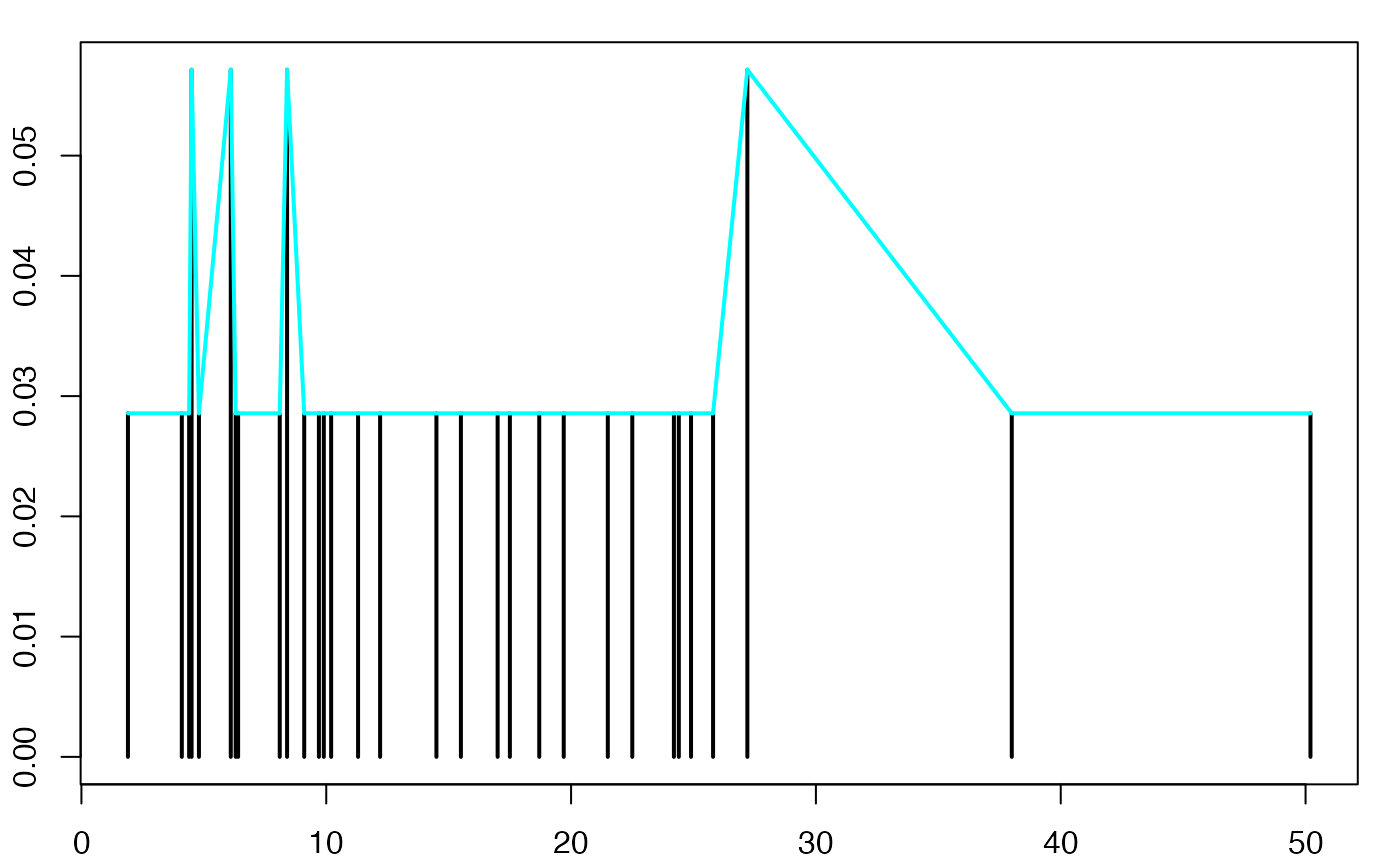
#suppressWarnings(par(oldpar))
pdf(file = paste(Chemin,"polyfrenew",varN,".pdf",sep=""),
    width = 8, height = 7, onefile = TRUE, family = "Helvetica",
    title = "Diagramme en bâtons des fréquences et polygone des fréquences", paper = "special", colormodel = colmodel)
par(mar = c(2, 2, 1, 1) + 0.1, mgp = c(2, 1, 0))
plot(xi,ni/sum(ni),type='h',xlab="",ylab="",lwd=2,ylim=c(0,max(ni/sum(ni))))
segments(xi[-length(xi)],ni[-length(xi)]/sum(ni),xi[-1],ni[-1]/sum(ni),lwd=2,col="#00FFFF")
dev.off()
#> agg_png
#>       2
Diagramme en bâtons des effectifs cumulés et polygone des effectifs cumulés
nisum <- rep(ni[1],length(ni))
for (iii in 2:length(ni))
{
  nisum[iii] <- nisum[iii-1]+ni[iii]
}

oldpar <- par()
par(mar = c(2, 2, 1, 1) + 0.1, mgp=c(2,1,0))
plot(xi,nisum,type='h',xlab="",ylab="",lwd=2,ylim=c(0,max(nisum))) #,xaxt="n"
segments(xi[-length(xi)],nisum[-length(xi)],xi[-1],nisum[-1],lwd=2,col="#00FFFF")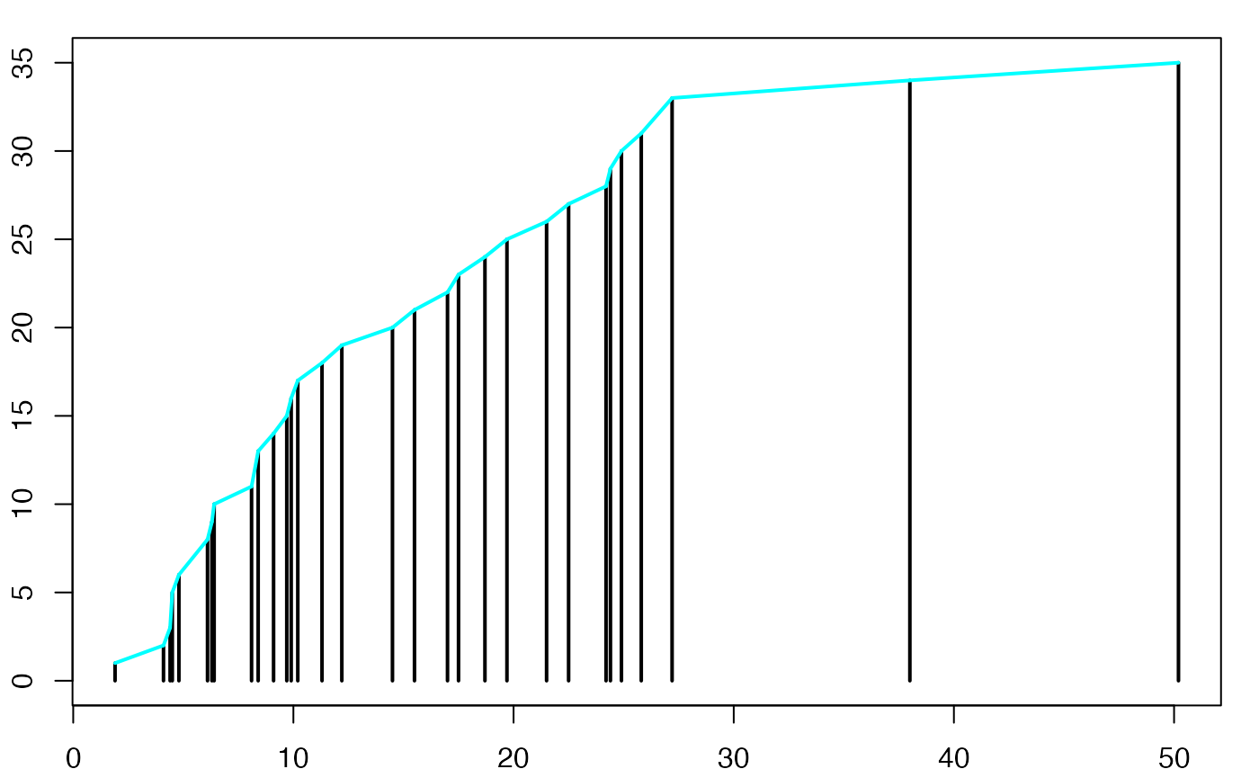
#suppressWarnings(par(oldpar))
pdf(file = paste(Chemin,"polyeffcumnew",varN,".pdf",sep=""),
    width = 8, height = 7, onefile = TRUE, family = "Helvetica",
    title = "Diagramme en bâtons des effectifs cumulés et polygone des effectifs cumulés", paper = "special", colormodel = colmodel)
par(mar = c(2, 2, 1, 1) + 0.1, mgp = c(2, 1, 0))
plot(xi,nisum,type='h',xlab="",ylab="",lwd=2,ylim=c(0,max(nisum))) #,xaxt="n"
segments(xi[-length(xi)],nisum[-length(xi)],xi[-1],nisum[-1],lwd=2,col="#00FFFF")
dev.off()
#> agg_png
#>       2
Diagramme en bâtons des fréquences cumulées
oldpar <- par()
par(mar = c(2, 2, 1, 1) + 0.1, mgp=c(2,1,0))
plot(xi,nisum/sum(ni),type='h',xlab="",ylab="",lwd=2,ylim=c(0,max(nisum/sum(ni))))  #,xaxt="n"
#suppressWarnings(par(oldpar))
pdf(file = paste(Chemin,"frecumnew",varN,".pdf",sep=""),
    width = 8, height = 7, onefile = TRUE, family = "Helvetica",
    title = "Diagramme en bâtons des fréquences cumulées", paper = "special", colormodel = colmodel)
par(mar = c(2, 2, 1, 1) + 0.1, mgp = c(2, 1, 0))
plot(xi,nisum/sum(ni),type='h',xlab="",ylab="",lwd=2,ylim=c(0,max(nisum/sum(ni))))  #,xaxt="n"
dev.off()
#> agg_png
#>       2
Diagramme en bâtons des effectifs cumulés
oldpar <- par()
par(mar = c(2, 2, 1, 1) + 0.1, mgp=c(2,1,0))
plot(xi,nisum,type='h',xlab="",ylab="",lwd=2,ylim=c(0,max(nisum))) #,xaxt="n"
#suppressWarnings(par(oldpar))
pdf(file = paste(Chemin,"effcumnew",varN,".pdf",sep=""),
    width = 8, height = 7, onefile = TRUE, family = "Helvetica",
    title = "Diagramme en bâtons des effectifs cumulés", paper = "special", colormodel = colmodel)
par(mar = c(2, 2, 1, 1) + 0.1, mgp = c(2, 1, 0))
plot(xi,nisum,type='h',xlab="",ylab="",lwd=2,ylim=c(0,max(nisum))) #,xaxt="n"
dev.off()
#> agg_png
#> 2Histogramme des fréquences
oldpar <- par()
par(mar = c(2, 2, 1, 1) + 0.1, mgp=c(2,1,0))
histofre <- hist(data3,breaks=breaks0,main="",freq=F,xlab="",ylab="",lwd=2,density=10)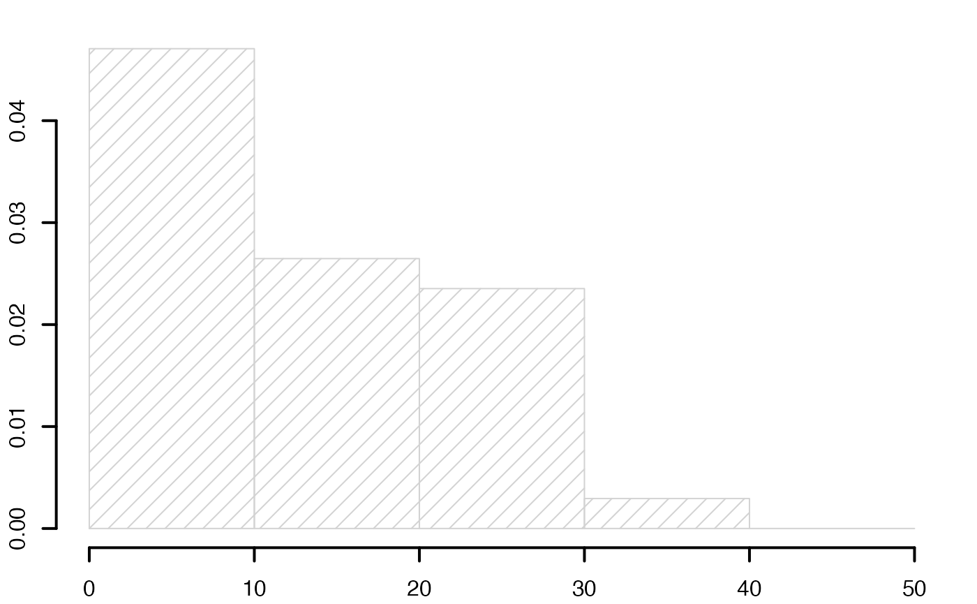
#suppressWarnings(par(oldpar))
Chemin <- "~/Documents/Recherche/DeBoeck/Graphes/Donnees/"
colmodel="cmyk"
pdf(file = paste(Chemin,"histofrenew",varN,".pdf",sep=""),
    width = 8, height = 7, onefile = TRUE, family = "Helvetica",
    title = "Histogramme des fréquences", paper = "special", colormodel = colmodel)
par(mar = c(2, 2, 1, 1) + 0.1, mgp = c(2, 1, 0))
histofre <- hist(data3,breaks=breaks0,main="",freq=F,xlab="",ylab="",lwd=2,density=10)
dev.off()
#> agg_png
#>       2
Histogramme des fréquences et polygone des fréquences
oldpar <- par()
par(mar = c(2, 2, 1, 1) + 0.1, mgp=c(2,1,0))
histofre <- hist(data3,breaks=breaks0,main="",freq=F,xlab="",ylab="",lwd=2,density=10)
segments(histofre$mids[-(length(breaks0)-1)],histofre$density[-(length(breaks0)-1)],histofre$mids[-1],histofre$density[-1],lwd=2,col="#00FFFF")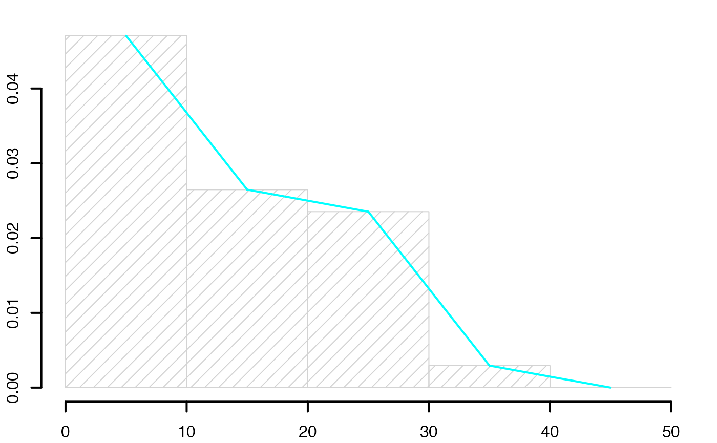
#suppressWarnings(par(oldpar))
Chemin <- "~/Documents/Recherche/DeBoeck/Graphes/Donnees/"
colmodel="cmyk"
pdf(file = paste(Chemin,"histopolfrenew",varN,".pdf",sep=""),
    width = 8, height = 7, onefile = TRUE, family = "Helvetica",
    title = "Histogramme des fréquences et polygone des fréquences", paper = "special", colormodel = colmodel)
par(mar = c(2, 2, 1, 1) + 0.1, mgp = c(2, 1, 0))
histofre <- hist(data3,breaks=breaks0,main="",freq=F,xlab="",ylab="",lwd=2,density=10)
segments(histofre$mids[-(length(breaks0)-1)],histofre$density[-(length(breaks0)-1)],histofre$mids[-1],histofre$density[-1],lwd=2,col="#00FFFF")
dev.off()
#> agg_png
#>       2
Histogramme des fréquences cumulés
data4 <- rep((breaks0[-length(breaks0)]+diff(breaks0)/2),cumsum(table(cut(var1,breaks0))))
table(data4)
#> data4
#>  5 15 25 35 45
#> 16 25 33 34 34

oldpar <- par()
par(mar = c(2, 2, 1, 1) + 0.1, mgp=c(2,1,0))
histofrecum <- hist(data4,breaks=breaks0,main="",freq=F,xlab="",ylab="",lwd=2,yaxt="n",density=10)
axis(2,at=c(0,.2,.4,.6,.8,1)*max(histofrecum$dens),labels=c(0,.2,.4,.6,.8,1),lwd=2)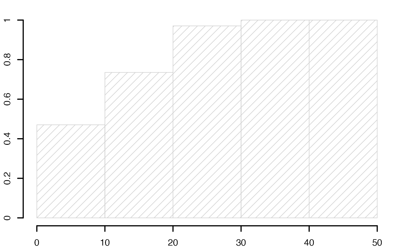
#suppressWarnings(par(oldpar))
Chemin <- "~/Documents/Recherche/DeBoeck/Graphes/Donnees/"
colmodel="cmyk"
pdf(file = paste(Chemin,"histofrecumnew",varN,".pdf",sep=""),
    width = 8, height = 7, onefile = TRUE, family = "Helvetica",
    title = "Histogramme des fréquences cumulés", paper = "special", colormodel = colmodel)
par(mar = c(2, 2, 1, 1) + 0.1, mgp = c(2, 1, 0))
histofrecum <- hist(data4,breaks=breaks0,main="",freq=F,xlab="",ylab="",lwd=2,yaxt="n",density=10)
axis(2,at=c(0,.2,.4,.6,.8,1)*max(histofrecum$dens),labels=c(0,.2,.4,.6,.8,1),lwd=2)
dev.off()
#> agg_png
#>       2
Histogramme des fréquences cumulées et polygone des fréquences cumulées
oldpar <- par()
par(mar = c(2, 2, 1, 1) + 0.1, mgp=c(2,1,0))
histofrecum <- hist(data4,breaks=breaks0,main="",freq=F,xlab="",ylab="",lwd=2,yaxt="n",density=10)
segments(histofrecum$mids[-(length(breaks0)-1)],histofrecum$density[-(length(breaks0)-1)],histofrecum$mids[-1],histofrecum$density[-1],lwd=2,col="#00FFFF")
axis(2,at=c(0,.2,.4,.6,.8,1)*max(histofrecum$dens),labels=c(0,.2,.4,.6,.8,1),lwd=2)
#suppressWarnings(par(oldpar))
pdf(file = paste(Chemin,"histopolfrecumnew",varN,".pdf",sep=""),
    width = 8, height = 7, onefile = TRUE, family = "Helvetica",
    title = "Histogramme des fréquences cumulées et polygone des fréquences cumulées", paper = "special", colormodel = colmodel)
par(mar = c(2, 2, 1, 1) + 0.1, mgp = c(2, 1, 0))
histofrecum <- hist(data4,breaks=breaks0,main="",freq=F,xlab="",ylab="",lwd=2,yaxt="n",density=10)
segments(histofrecum$mids[-(length(breaks0)-1)],histofrecum$density[-(length(breaks0)-1)],histofrecum$mids[-1],histofrecum$density[-1],lwd=2,col="#00FFFF")
axis(2,at=c(0,.2,.4,.6,.8,1)*max(histofrecum$dens),labels=c(0,.2,.4,.6,.8,1),lwd=2)
dev.off()
#> agg_png
#>       2
Histogramme des effectifs cumulés et polygone des effectifs cumulés
oldpar <- par()
par(mar = c(2, 2, 1, 1) + 0.1, mgp=c(2,1,0))
histoeffcum <- hist(data4,breaks=breaks0,main="",freq=T,xlab="",ylab="",lwd=2,density=10)   #,yaxt="n"
segments(histoeffcum$mids[-(length(breaks0)-1)],histoeffcum$counts[-(length(breaks0)-1)],histoeffcum$mids[-1],histoeffcum$counts[-1],lwd=2,col="#00FFFF")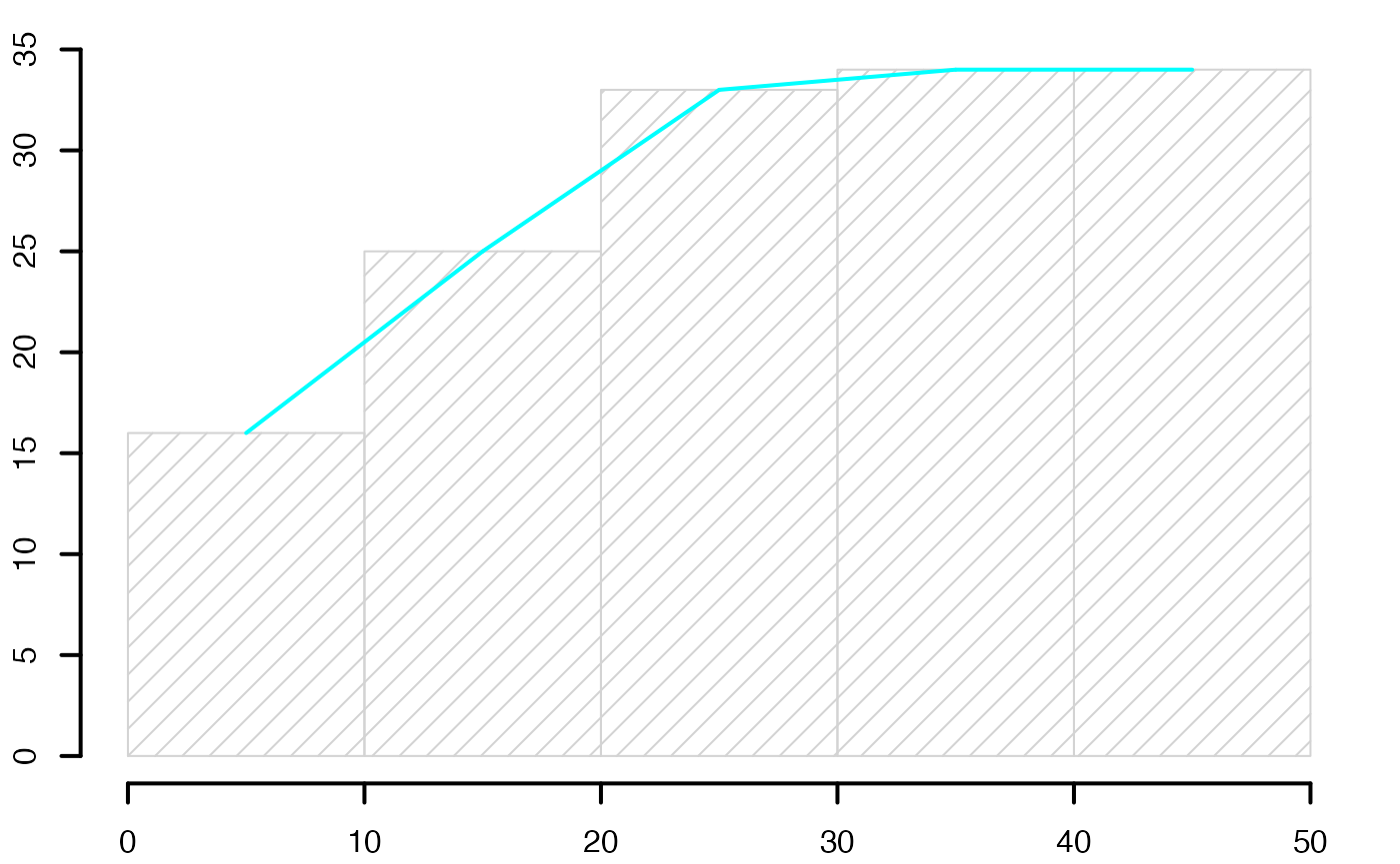
#axis(2,at=c(0,.2,.4,.6,.8,1)*length(data3),labels=c(0,.2,.4,.6,.8,1)*length(data3),lwd=2)
#suppressWarnings(par(oldpar))
pdf(file = paste(Chemin,"histopoleffcumnew",varN,".pdf",sep=""),
    width = 8, height = 7, onefile = TRUE, family = "Helvetica",
    title = "Histogramme des effectifs cumulés et polygone des effectifs cumulés", paper = "special", colormodel = colmodel)
par(mar = c(2, 2, 1, 1) + 0.1, mgp = c(2, 1, 0))
histoeffcum <- hist(data4,breaks=breaks0,main="",freq=T,xlab="",ylab="",lwd=2,density=10)     #,yaxt="n"
segments(histoeffcum$mids[-(length(breaks0)-1)],histoeffcum$counts[-(length(breaks0)-1)],histoeffcum$mids[-1],histoeffcum$counts[-1],lwd=2,col="#00FFFF")
#axis(2,at=c(0,.2,.4,.6,.8,1)*length(data3),labels=c(0,.2,.4,.6,.8,1)*length(data3),lwd=2)
dev.off()
#> agg_png
#>       2
Partiel Hommes
data(Europe)

var1<- Europe$Partiel_H
varN <- "_H"

xi <- unique(sort(var1))
ni <- as.vector(table(var1))

data2 <- cbind(xi,ni)
Diagramme en bâtons des effectifs
oldpar <- par()
par(mar = c(2, 2, 1, 1) + 0.1, mgp=c(2,1,0))
plot(xi,ni,type='h',xlab="",ylab="",lwd=2,ylim=c(0,max(ni))) #,xaxt="n"
#axis(1, at = 1:6, labels = c(1:5,6))
#axis(1, at = 1:6, labels = c(1:5,"6 et plus"))
#suppressWarnings(par(oldpar))
Chemin <- "~/Documents/Recherche/DeBoeck/Graphes/Donnees/"
colmodel="cmyk"
pdf(file = paste(Chemin,"batoneffnew",varN,".pdf",sep=""),
    width = 8, height = 7, onefile = TRUE, family = "Helvetica",
    title = "Diagramme en bâtons des effectifs", paper = "special", colormodel = colmodel)
par(mar = c(2, 2, 1, 1) + 0.1, mgp = c(2, 1, 0))
plot(xi,ni,type='h',xlab="",ylab="",lwd=2,ylim=c(0,max(ni))) #,xaxt="n"
dev.off()
#> agg_png
#>       2
Diagramme en bâtons des fréquences
oldpar <- par()
par(mar = c(2, 2, 1, 1) + 0.1, mgp=c(2,1,0))
plot(xi,ni/sum(ni),type='h',xlab="",ylab="",lwd=2,ylim=c(0,max(ni/sum(ni))))   #,xaxt="n"
#suppressWarnings(par(oldpar))
pdf(file = paste(Chemin,"batonfrenew",varN,".pdf",sep=""),
    width = 8, height = 7, onefile = TRUE, family = "Helvetica",
    title = "Diagramme en bâtons des fréquences", paper = "special", colormodel = colmodel)
par(mar = c(2, 2, 1, 1) + 0.1, mgp = c(2, 1, 0))
plot(xi,ni/sum(ni),type='h',xlab="",ylab="",lwd=2,ylim=c(0,max(ni/sum(ni))))   #,xaxt="n"
dev.off()
#> agg_png
#>       2
Diagramme en bâtons des effectifs et polygone des effectifs
oldpar <- par()
par(mar = c(2, 2, 1, 1) + 0.1, mgp=c(2,1,0))
plot(xi,ni,type='h',xlab="",ylab="",lwd=2,ylim=c(0,max(ni))) #,xaxt="n"
segments(xi[-length(xi)],ni[-length(xi)],xi[-1],ni[-1],lwd=2,col="#00FFFF")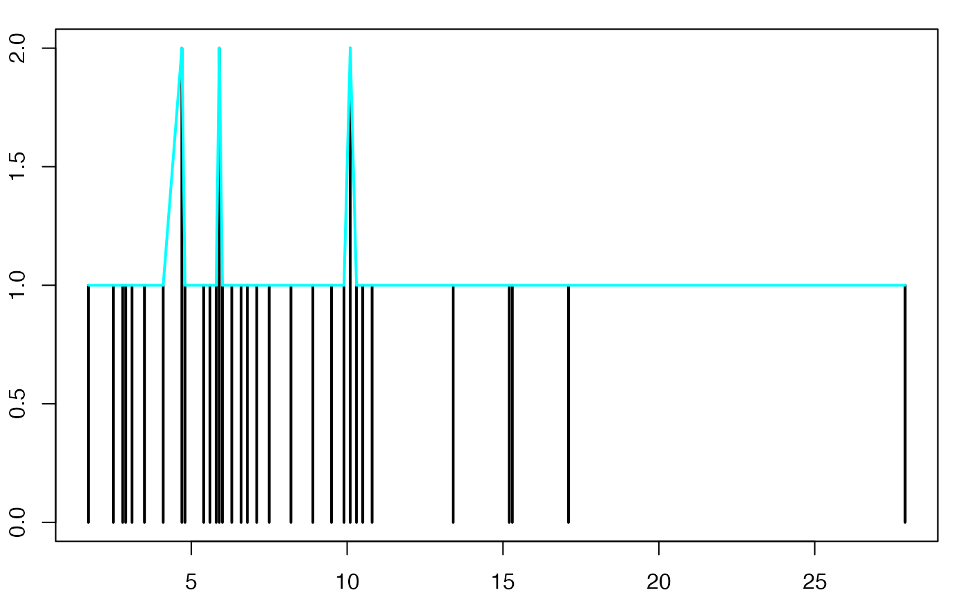
#suppressWarnings(par(oldpar))
pdf(file = paste(Chemin,"polyeffnew",varN,".pdf",sep=""),
    width = 8, height = 7, onefile = TRUE, family = "Helvetica",
    title = "Diagramme en bâtons des effectifs et polygone des effectifs", paper = "special", colormodel = colmodel)
par(mar = c(2, 2, 1, 1) + 0.1, mgp = c(2, 1, 0))
plot(xi,ni,type='h',xlab="",ylab="",lwd=2,ylim=c(0,max(ni))) #,xaxt="n"
segments(xi[-length(xi)],ni[-length(xi)],xi[-1],ni[-1],lwd=2,col="#00FFFF")
dev.off()
#> agg_png
#>       2
Diagramme en bâtons des fréquences et polygone des fréquences
oldpar <- par()
par(mar = c(2, 2, 1, 1) + 0.1, mgp=c(2,1,0))
plot(xi,ni/sum(ni),type='h',xlab="",ylab="",lwd=2,ylim=c(0,max(ni/sum(ni))))
segments(xi[-length(xi)],ni[-length(xi)]/sum(ni),xi[-1],ni[-1]/sum(ni),lwd=2,col="#00FFFF")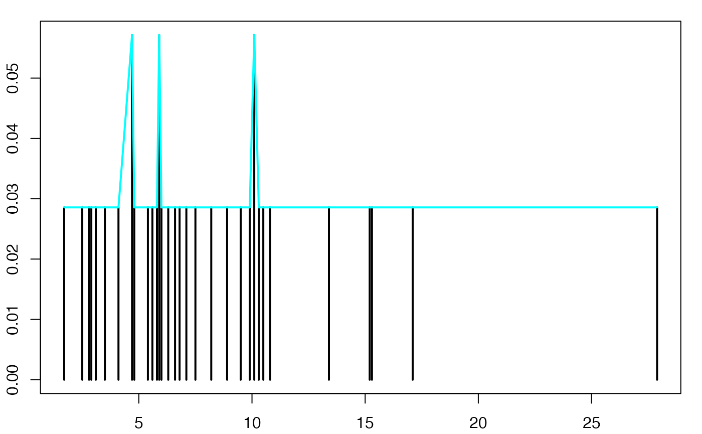
#suppressWarnings(par(oldpar))
pdf(file = paste(Chemin,"polyfrenew",varN,".pdf",sep=""),
    width = 8, height = 7, onefile = TRUE, family = "Helvetica",
    title = "Diagramme en bâtons des fréquences et polygone des fréquences", paper = "special", colormodel = colmodel)
par(mar = c(2, 2, 1, 1) + 0.1, mgp = c(2, 1, 0))
plot(xi,ni/sum(ni),type='h',xlab="",ylab="",lwd=2,ylim=c(0,max(ni/sum(ni))))
segments(xi[-length(xi)],ni[-length(xi)]/sum(ni),xi[-1],ni[-1]/sum(ni),lwd=2,col="#00FFFF")
dev.off()
#> agg_png
#>       2
Diagramme en bâtons des effectifs cumulés et polygone des effectifs cumulés
nisum <- rep(ni[1],length(ni))
for (iii in 2:length(ni))
{
  nisum[iii] <- nisum[iii-1]+ni[iii]
}

oldpar <- par()
par(mar = c(2, 2, 1, 1) + 0.1, mgp=c(2,1,0))
plot(xi,nisum,type='h',xlab="",ylab="",lwd=2,ylim=c(0,max(nisum))) #,xaxt="n"
segments(xi[-length(xi)],nisum[-length(xi)],xi[-1],nisum[-1],lwd=2,col="#00FFFF")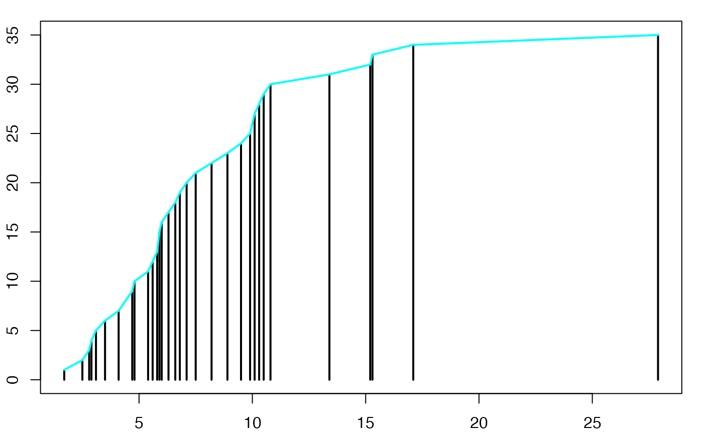
#suppressWarnings(par(oldpar))
pdf(file = paste(Chemin,"polyeffcumnew",varN,".pdf",sep=""),
    width = 8, height = 7, onefile = TRUE, family = "Helvetica",
    title = "Diagramme en bâtons des effectifs cumulés et polygone des effectifs cumulés", paper = "special", colormodel = colmodel)
par(mar = c(2, 2, 1, 1) + 0.1, mgp = c(2, 1, 0))
plot(xi,nisum,type='h',xlab="",ylab="",lwd=2,ylim=c(0,max(nisum))) #,xaxt="n"
segments(xi[-length(xi)],nisum[-length(xi)],xi[-1],nisum[-1],lwd=2,col="#00FFFF")
dev.off()
#> agg_png
#>       2
Diagramme en bâtons des fréquences cumulées
oldpar <- par()
par(mar = c(2, 2, 1, 1) + 0.1, mgp=c(2,1,0))
plot(xi,nisum/sum(ni),type='h',xlab="",ylab="",lwd=2,ylim=c(0,max(nisum/sum(ni))))  #,xaxt="n"
#suppressWarnings(par(oldpar))
pdf(file = paste(Chemin,"frecumnew",varN,".pdf",sep=""),
    width = 8, height = 7, onefile = TRUE, family = "Helvetica",
    title = "Diagramme en bâtons des fréquences cumulées", paper = "special", colormodel = colmodel)
par(mar = c(2, 2, 1, 1) + 0.1, mgp = c(2, 1, 0))
plot(xi,nisum/sum(ni),type='h',xlab="",ylab="",lwd=2,ylim=c(0,max(nisum/sum(ni))))  #,xaxt="n"
dev.off()
#> agg_png
#>       2
Diagramme en bâtons des effectifs cumulés
oldpar <- par()
par(mar = c(2, 2, 1, 1) + 0.1, mgp=c(2,1,0))
plot(xi,nisum,type='h',xlab="",ylab="",lwd=2,ylim=c(0,max(nisum))) #,xaxt="n"
#suppressWarnings(par(oldpar))
pdf(file = paste(Chemin,"effcumnew",varN,".pdf",sep=""),
    width = 8, height = 7, onefile = TRUE, family = "Helvetica",
    title = "Diagramme en bâtons des effectifs cumulés", paper = "special", colormodel = colmodel)
par(mar = c(2, 2, 1, 1) + 0.1, mgp = c(2, 1, 0))
plot(xi,nisum,type='h',xlab="",ylab="",lwd=2,ylim=c(0,max(nisum))) #,xaxt="n"
dev.off()
#> agg_png
#> 2Histogramme des fréquences
oldpar <- par()
par(mar = c(2, 2, 1, 1) + 0.1, mgp=c(2,1,0))
histofre <- hist(data3,breaks=breaks0,main="",freq=F,xlab="",ylab="",lwd=2,density=10)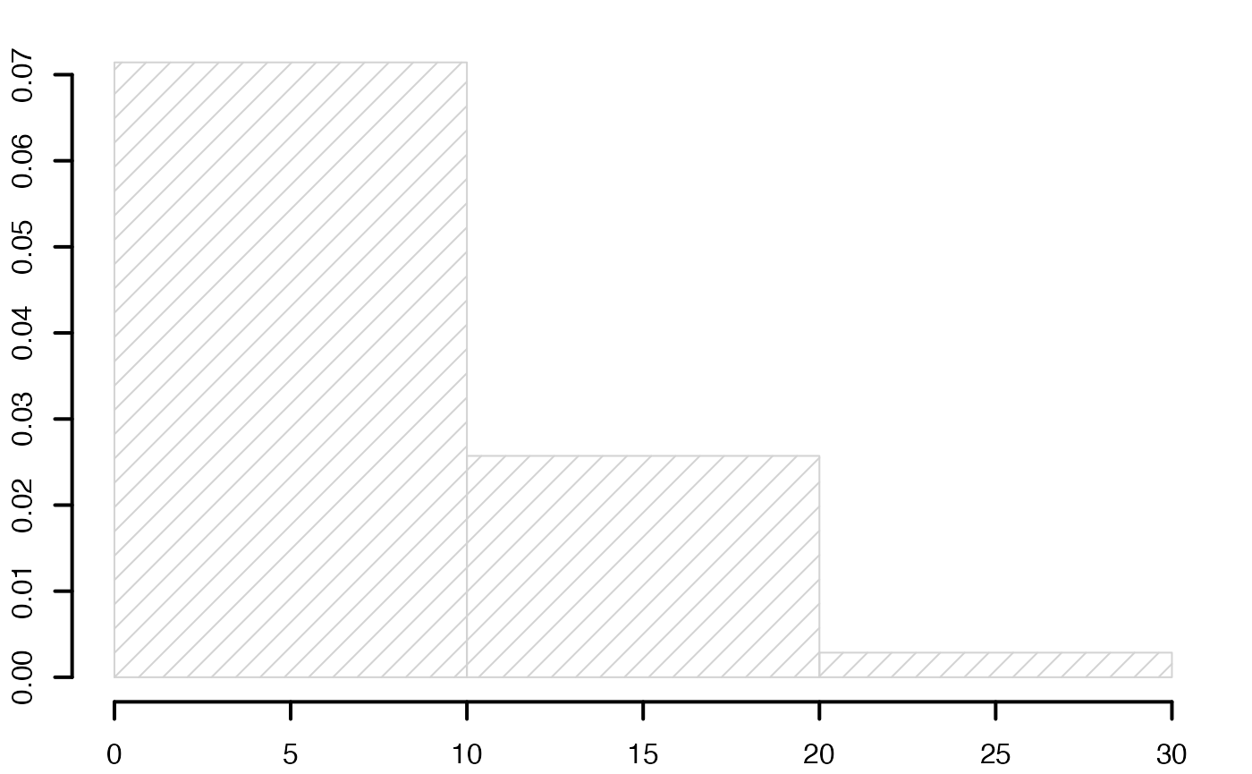
#suppressWarnings(par(oldpar))
Chemin <- "~/Documents/Recherche/DeBoeck/Graphes/Donnees/"
colmodel="cmyk"
pdf(file = paste(Chemin,"histofrenew",varN,".pdf",sep=""),
    width = 8, height = 7, onefile = TRUE, family = "Helvetica",
    title = "Histogramme des fréquences", paper = "special", colormodel = colmodel)
par(mar = c(2, 2, 1, 1) + 0.1, mgp = c(2, 1, 0))
histofre <- hist(data3,breaks=breaks0,main="",freq=F,xlab="",ylab="",lwd=2,density=10)
dev.off()
#> agg_png
#>       2
Histogramme des fréquences et polygone des fréquences
oldpar <- par()
par(mar = c(2, 2, 1, 1) + 0.1, mgp=c(2,1,0))
histofre <- hist(data3,breaks=breaks0,main="",freq=F,xlab="",ylab="",lwd=2,density=10)
segments(histofre$mids[-(length(breaks0)-1)],histofre$density[-(length(breaks0)-1)],histofre$mids[-1],histofre$density[-1],lwd=2,col="#00FFFF")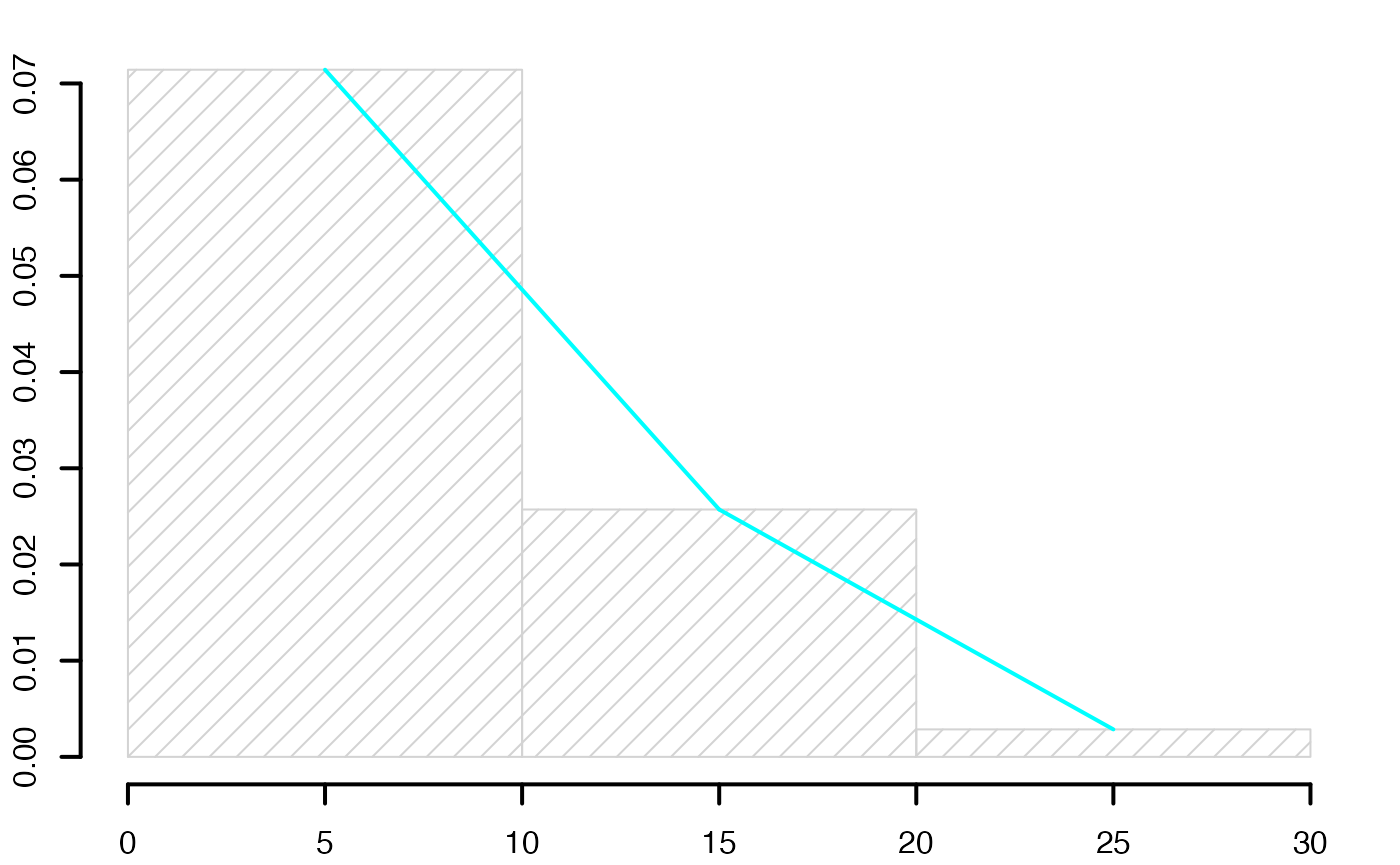
#suppressWarnings(par(oldpar))
pdf(file = paste(Chemin,"histopolfrenew",varN,".pdf",sep=""),
    width = 8, height = 7, onefile = TRUE, family = "Helvetica",
    title = "Histogramme des fréquences et polygone des fréquences", paper = "special", colormodel = colmodel)
par(mar = c(2, 2, 1, 1) + 0.1, mgp = c(2, 1, 0))
histofre <- hist(data3,breaks=breaks0,main="",freq=F,xlab="",ylab="",lwd=2,density=10)
segments(histofre$mids[-(length(breaks0)-1)],histofre$density[-(length(breaks0)-1)],histofre$mids[-1],histofre$density[-1],lwd=2,col="#00FFFF")
dev.off()
#> agg_png
#>       2
Histogramme des fréquences cumulés
data4 <- rep((breaks0[-length(breaks0)]+diff(breaks0)/2)
             ,cumsum(table(cut(var1,breaks0))))
table(data4)
#> data4
#>  5 15 25
#> 25 34 35
oldpar <- par()
par(mar = c(2, 2, 1, 1) + 0.1, mgp=c(2,1,0))
histofrecum <- hist(data4,breaks=breaks0,main="",freq=F,xlab="",ylab="",lwd=2,yaxt="n",density=10)
axis(2,at=c(0,.2,.4,.6,.8,1)*max(histofrecum$dens),labels=c(0,.2,.4,.6,.8,1),lwd=2)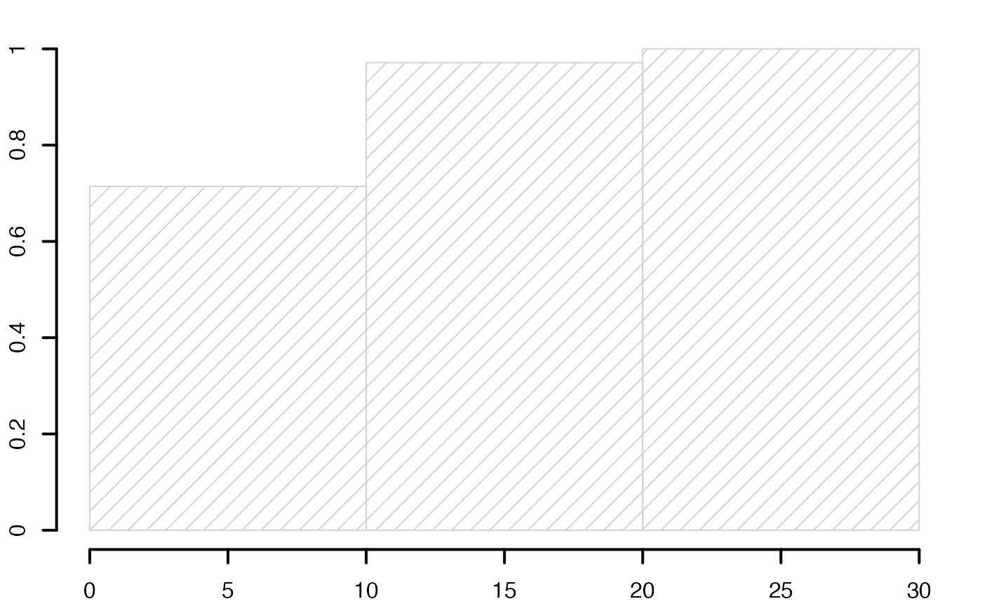
#suppressWarnings(par(oldpar))
pdf(file = paste(Chemin,"histofrecumnew",varN,".pdf",sep=""),
    width = 8, height = 7, onefile = TRUE, family = "Helvetica",
    title = "Histogramme des fréquences cumulés", paper = "special", colormodel = colmodel)
par(mar = c(2, 2, 1, 1) + 0.1, mgp = c(2, 1, 0))
histofrecum <- hist(data4,breaks=breaks0,main="",freq=F,xlab="",ylab="",lwd=2,yaxt="n",density=10)
axis(2,at=c(0,.2,.4,.6,.8,1)*max(histofrecum$dens),labels=c(0,.2,.4,.6,.8,1),lwd=2)
dev.off()
#> agg_png
#>       2
Histogramme des fréquences cumulées et polygone des fréquences cumulées
oldpar <- par()
par(mar = c(2, 2, 1, 1) + 0.1, mgp=c(2,1,0))
histofrecum <- hist(data4,breaks=breaks0,main="",freq=F,xlab="",ylab="",lwd=2,yaxt="n",density=10)
segments(histofrecum$mids[-(length(breaks0)-1)],histofrecum$density[-(length(breaks0)-1)],histofrecum$mids[-1],histofrecum$density[-1],lwd=2,col="#00FFFF")
axis(2,at=c(0,.2,.4,.6,.8,1)*max(histofrecum$dens),labels=c(0,.2,.4,.6,.8,1),lwd=2)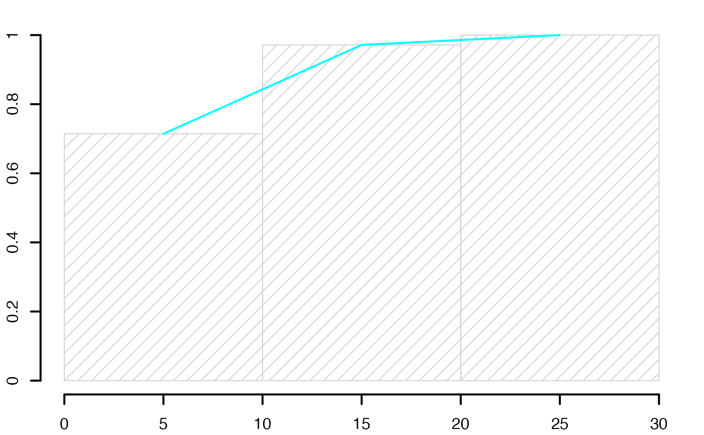
#suppressWarnings(par(oldpar))
pdf(file = paste(Chemin,"histopolfrecumnew",varN,".pdf",sep=""),
    width = 8, height = 7, onefile = TRUE, family = "Helvetica",
    title = "Histogramme des fréquences cumulées et polygone des fréquences cumulées", paper = "special", colormodel = colmodel)
par(mar = c(2, 2, 1, 1) + 0.1, mgp = c(2, 1, 0))
histofrecum <- hist(data4,breaks=breaks0,main="",freq=F,xlab="",ylab="",lwd=2,yaxt="n",density=10)
segments(histofrecum$mids[-(length(breaks0)-1)],histofrecum$density[-(length(breaks0)-1)],histofrecum$mids[-1],histofrecum$density[-1],lwd=2,col="#00FFFF")
axis(2,at=c(0,.2,.4,.6,.8,1)*max(histofrecum$dens),labels=c(0,.2,.4,.6,.8,1),lwd=2)
dev.off()
#> agg_png
#>       2
Histogramme des effectifs cumulés et polygone des effectifs cumulés
oldpar <- par()
par(mar = c(2, 2, 1, 1) + 0.1, mgp=c(2,1,0))
histoeffcum <- hist(data4,breaks=breaks0,main="",freq=T,xlab="",ylab="",lwd=2,density=10)   #,yaxt="n"
segments(histoeffcum$mids[-(length(breaks0)-1)],histoeffcum$counts[-(length(breaks0)-1)],histoeffcum$mids[-1],histoeffcum$counts[-1],lwd=2,col="#00FFFF")
#axis(2,at=c(0,.2,.4,.6,.8,1)*length(data3),labels=c(0,.2,.4,.6,.8,1)*length(data3),lwd=2)
#suppressWarnings(par(oldpar))
pdf(file = paste(Chemin,"histopoleffcumnew",varN,".pdf",sep=""),
    width = 8, height = 7, onefile = TRUE, family = "Helvetica",
    title = "Histogramme des effectifs cumulés et polygone des effectifs cumulés", paper = "special", colormodel = colmodel)
par(mar = c(2, 2, 1, 1) + 0.1, mgp = c(2, 1, 0))
histoeffcum <- hist(data4,breaks=breaks0,main="",freq=T,xlab="",ylab="",lwd=2,density=10)     #,yaxt="n"
segments(histoeffcum$mids[-(length(breaks0)-1)],histoeffcum$counts[-(length(breaks0)-1)],histoeffcum$mids[-1],histoeffcum$counts[-1],lwd=2,col="#00FFFF")
#axis(2,at=c(0,.2,.4,.6,.8,1)*length(data3),labels=c(0,.2,.4,.6,.8,1)*length(data3),lwd=2)
dev.off()
#> agg_png
#>       2
Partiel Femmes
data(Europe)

var1<- Europe$Partiel_F
varN <- "_F"

xi <- unique(sort(var1))
ni <- as.vector(table(var1))

data2 <- cbind(xi,ni)
Diagramme en bâtons des effectifs
oldpar <- par()
par(mar = c(2, 2, 1, 1) + 0.1, mgp=c(2,1,0))
plot(xi,ni,type='h',xlab="",ylab="",lwd=2,ylim=c(0,max(ni))) #,xaxt="n"
#axis(1, at = 1:6, labels = c(1:5,6))
#axis(1, at = 1:6, labels = c(1:5,"6 et plus"))
#suppressWarnings(par(oldpar))
Chemin <- "~/Documents/Recherche/DeBoeck/Graphes/Donnees/"
colmodel="cmyk"
pdf(file = paste(Chemin,"batoneffnew",varN,".pdf",sep=""),
    width = 8, height = 7, onefile = TRUE, family = "Helvetica",
    title = "Diagramme en bâtons des effectifs", paper = "special", colormodel = colmodel)
par(mar = c(2, 2, 1, 1) + 0.1, mgp = c(2, 1, 0))
plot(xi,ni,type='h',xlab="",ylab="",lwd=2,ylim=c(0,max(ni))) #,xaxt="n"
dev.off()
#> agg_png
#>       2
Diagramme en bâtons des fréquences
oldpar <- par()
par(mar = c(2, 2, 1, 1) + 0.1, mgp=c(2,1,0))
plot(xi,ni/sum(ni),type='h',xlab="",ylab="",lwd=2,ylim=c(0,max(ni/sum(ni))))   #,xaxt="n"
#suppressWarnings(par(oldpar))
pdf(file = paste(Chemin,"batonfrenew",varN,".pdf",sep=""),
    width = 8, height = 7, onefile = TRUE, family = "Helvetica",
    title = "Diagramme en bâtons des fréquences", paper = "special", colormodel = colmodel)
par(mar = c(2, 2, 1, 1) + 0.1, mgp = c(2, 1, 0))
plot(xi,ni/sum(ni),type='h',xlab="",ylab="",lwd=2,ylim=c(0,max(ni/sum(ni))))   #,xaxt="n"
dev.off()
#> agg_png
#>       2
Diagramme en bâtons des effectifs et polygone des effectifs
oldpar <- par()
par(mar = c(2, 2, 1, 1) + 0.1, mgp=c(2,1,0))
plot(xi,ni,type='h',xlab="",ylab="",lwd=2,ylim=c(0,max(ni))) #,xaxt="n"
segments(xi[-length(xi)],ni[-length(xi)],xi[-1],ni[-1],lwd=2,col="#00FFFF")
#suppressWarnings(par(oldpar))
pdf(file = paste(Chemin,"polyeffnew",varN,".pdf",sep=""),
    width = 8, height = 7, onefile = TRUE, family = "Helvetica",
    title = "Diagramme en bâtons des effectifs et polygone des effectifs", paper = "special", colormodel = colmodel)
par(mar = c(2, 2, 1, 1) + 0.1, mgp = c(2, 1, 0))
plot(xi,ni,type='h',xlab="",ylab="",lwd=2,ylim=c(0,max(ni))) #,xaxt="n"
segments(xi[-length(xi)],ni[-length(xi)],xi[-1],ni[-1],lwd=2,col="#00FFFF")
dev.off()
#> agg_png
#>       2
Diagramme en bâtons des fréquences et polygone des fréquences
oldpar <- par()
par(mar = c(2, 2, 1, 1) + 0.1, mgp=c(2,1,0))
plot(xi,ni/sum(ni),type='h',xlab="",ylab="",lwd=2,ylim=c(0,max(ni/sum(ni))))
segments(xi[-length(xi)],ni[-length(xi)]/sum(ni),xi[-1],ni[-1]/sum(ni),lwd=2,col="#00FFFF")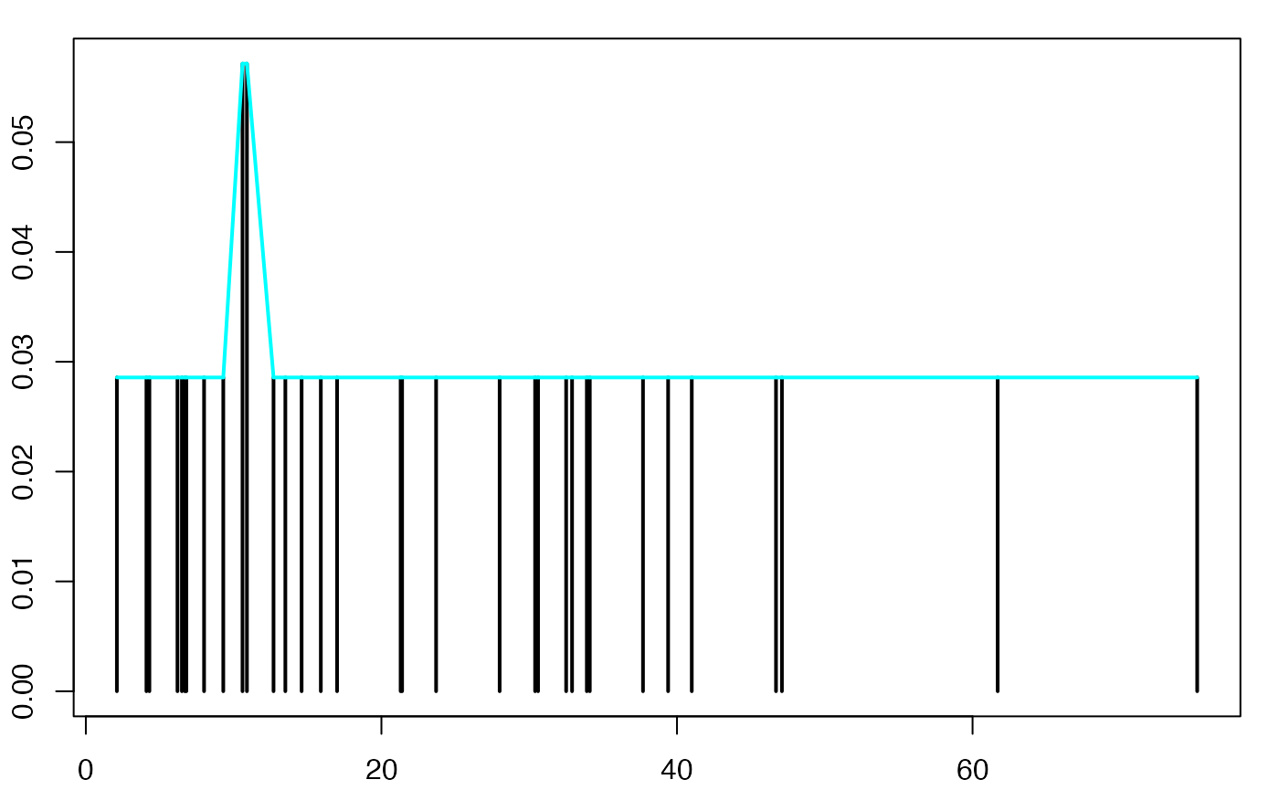
#suppressWarnings(par(oldpar))
pdf(file = paste(Chemin,"polyfrenew",varN,".pdf",sep=""),
    width = 8, height = 7, onefile = TRUE, family = "Helvetica",
    title = "Diagramme en bâtons des fréquences et polygone des fréquences", paper = "special", colormodel = colmodel)
par(mar = c(2, 2, 1, 1) + 0.1, mgp = c(2, 1, 0))
plot(xi,ni/sum(ni),type='h',xlab="",ylab="",lwd=2,ylim=c(0,max(ni/sum(ni))))
segments(xi[-length(xi)],ni[-length(xi)]/sum(ni),xi[-1],ni[-1]/sum(ni),lwd=2,col="#00FFFF")
dev.off()
#> agg_png
#>       2
Diagramme en bâtons des effectifs cumulés et polygone des effectifs cumulés
nisum <- rep(ni[1],length(ni))
for (iii in 2:length(ni))
{
  nisum[iii] <- nisum[iii-1]+ni[iii]
}

oldpar <- par()
par(mar = c(2, 2, 1, 1) + 0.1, mgp=c(2,1,0))
plot(xi,nisum,type='h',xlab="",ylab="",lwd=2,ylim=c(0,max(nisum))) #,xaxt="n"
segments(xi[-length(xi)],nisum[-length(xi)],xi[-1],nisum[-1],lwd=2,col="#00FFFF")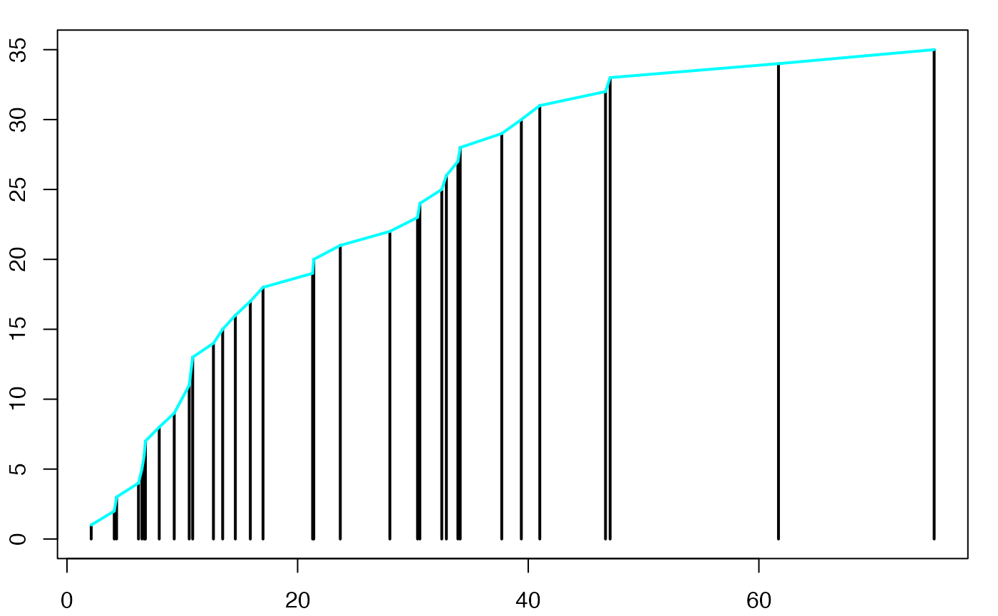
#suppressWarnings(par(oldpar))
pdf(file = paste(Chemin,"polyeffcumnew",varN,".pdf",sep=""),
    width = 8, height = 7, onefile = TRUE, family = "Helvetica",
    title = "Diagramme en bâtons des effectifs cumulés et polygone des effectifs cumulés", paper = "special", colormodel = colmodel)
par(mar = c(2, 2, 1, 1) + 0.1, mgp = c(2, 1, 0))
plot(xi,nisum,type='h',xlab="",ylab="",lwd=2,ylim=c(0,max(nisum))) #,xaxt="n"
segments(xi[-length(xi)],nisum[-length(xi)],xi[-1],nisum[-1],lwd=2,col="#00FFFF")
dev.off()
#> agg_png
#>       2
Diagramme en bâtons des fréquences cumulées
oldpar <- par()
par(mar = c(2, 2, 1, 1) + 0.1, mgp=c(2,1,0))
plot(xi,nisum/sum(ni),type='h',xlab="",ylab="",lwd=2,ylim=c(0,max(nisum/sum(ni))))  #,xaxt="n"
#suppressWarnings(par(oldpar))
pdf(file = paste(Chemin,"frecumnew",varN,".pdf",sep=""),
    width = 8, height = 7, onefile = TRUE, family = "Helvetica",
    title = "Diagramme en bâtons des fréquences cumulées", paper = "special", colormodel = colmodel)
par(mar = c(2, 2, 1, 1) + 0.1, mgp = c(2, 1, 0))
plot(xi,nisum/sum(ni),type='h',xlab="",ylab="",lwd=2,ylim=c(0,max(nisum/sum(ni))))  #,xaxt="n"
dev.off()
#> agg_png
#>       2
Diagramme en bâtons des effectifs cumulés
oldpar <- par()
par(mar = c(2, 2, 1, 1) + 0.1, mgp=c(2,1,0))
plot(xi,nisum,type='h',xlab="",ylab="",lwd=2,ylim=c(0,max(nisum))) #,xaxt="n"
#suppressWarnings(par(oldpar))
pdf(file = paste(Chemin,"effcumnew",varN,".pdf",sep=""),
    width = 8, height = 7, onefile = TRUE, family = "Helvetica",
    title = "Diagramme en bâtons des effectifs cumulés", paper = "special", colormodel = colmodel)
par(mar = c(2, 2, 1, 1) + 0.1, mgp = c(2, 1, 0))
plot(xi,nisum,type='h',xlab="",ylab="",lwd=2,ylim=c(0,max(nisum))) #,xaxt="n"
dev.off()
#> agg_png
#> 2Histogramme des fréquences
oldpar <- par()
par(mar = c(2, 2, 1, 1) + 0.1, mgp=c(2,1,0))
histofre <- hist(data3,breaks=breaks0,main="",freq=F,xlab="",ylab="",lwd=2,density=10)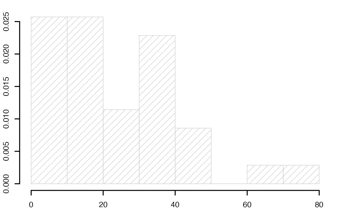
#suppressWarnings(par(oldpar))
Chemin <- "~/Documents/Recherche/DeBoeck/Graphes/Donnees/"
colmodel="cmyk"
pdf(file = paste(Chemin,"histofrenew",varN,".pdf",sep=""),
    width = 8, height = 7, onefile = TRUE, family = "Helvetica",
    title = "Histogramme des fréquences", paper = "special", colormodel = colmodel)
par(mar = c(2, 2, 1, 1) + 0.1, mgp = c(2, 1, 0))
histofre <- hist(data3,breaks=breaks0,main="",freq=F,xlab="",ylab="",lwd=2,density=10)
dev.off()
#> agg_png
#>       2
Histogramme des fréquences et polygone des fréquences
oldpar <- par()
par(mar = c(2, 2, 1, 1) + 0.1, mgp=c(2,1,0))
histofre <- hist(data3,breaks=breaks0,main="",freq=F,xlab="",ylab="",lwd=2,density=10)
segments(histofre$mids[-(length(breaks0)-1)],histofre$density[-(length(breaks0)-1)],histofre$mids[-1],histofre$density[-1],lwd=2,col="#00FFFF")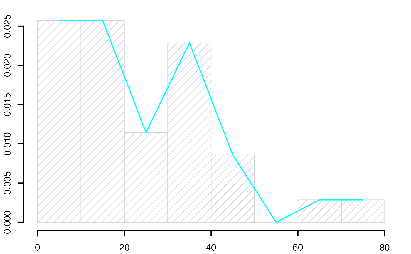
#suppressWarnings(par(oldpar))
pdf(file = paste(Chemin,"histopolfrenew",varN,".pdf",sep=""),
    width = 8, height = 7, onefile = TRUE, family = "Helvetica",
    title = "Histogramme des fréquences et polygone des fréquences", paper = "special", colormodel = colmodel)
par(mar = c(2, 2, 1, 1) + 0.1, mgp = c(2, 1, 0))
histofre <- hist(data3,breaks=breaks0,main="",freq=F,xlab="",ylab="",lwd=2,density=10)
segments(histofre$mids[-(length(breaks0)-1)],histofre$density[-(length(breaks0)-1)],histofre$mids[-1],histofre$density[-1],lwd=2,col="#00FFFF")
dev.off()
#> agg_png
#>       2
Histogramme des fréquences cumulés
data4 <- rep((breaks0[-length(breaks0)]+diff(breaks0)/2)
             ,cumsum(table(cut(var1,breaks0))))
table(data4)
#> data4
#>  5 15 25 35 45 55 65 75
#>  9 18 22 30 33 33 34 35

oldpar <- par()
par(mar = c(2, 2, 1, 1) + 0.1, mgp=c(2,1,0))
histofrecum <- hist(data4,breaks=breaks0,main="",freq=F,xlab="",ylab="",lwd=2,yaxt="n",density=10)
axis(2,at=c(0,.2,.4,.6,.8,1)*max(histofrecum$dens),labels=c(0,.2,.4,.6,.8,1),lwd=2)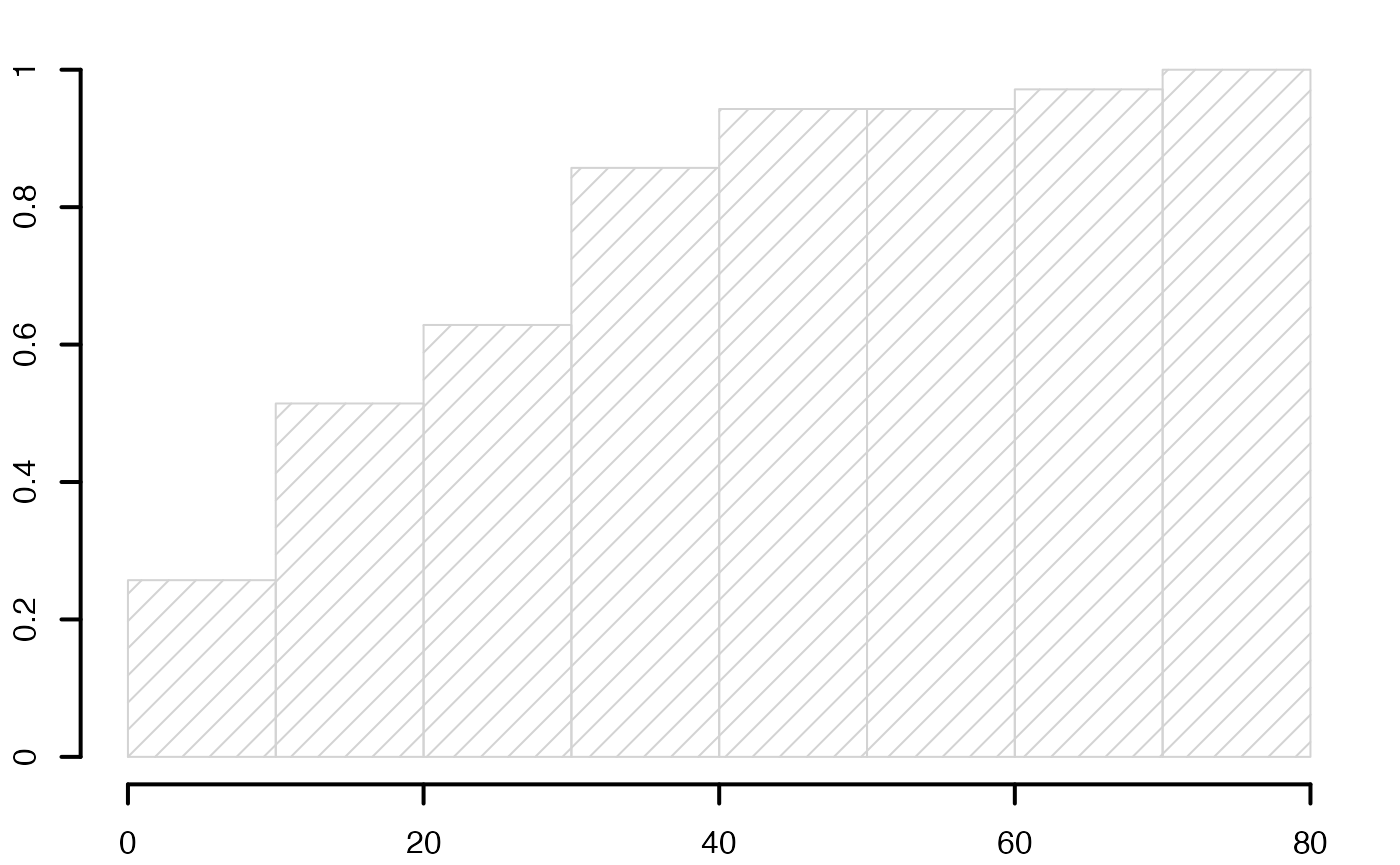
#suppressWarnings(par(oldpar))
pdf(file = paste(Chemin,"histofrecumnew",varN,".pdf",sep=""),
    width = 8, height = 7, onefile = TRUE, family = "Helvetica",
    title = "Histogramme des fréquences cumulés", paper = "special", colormodel = colmodel)
par(mar = c(2, 2, 1, 1) + 0.1, mgp = c(2, 1, 0))
histofrecum <- hist(data4,breaks=breaks0,main="",freq=F,xlab="",ylab="",lwd=2,yaxt="n",density=10)
axis(2,at=c(0,.2,.4,.6,.8,1)*max(histofrecum$dens),labels=c(0,.2,.4,.6,.8,1),lwd=2)
dev.off()
#> agg_png
#>       2
Histogramme des fréquences cumulées et polygone des fréquences cumulées
oldpar <- par()
par(mar = c(2, 2, 1, 1) + 0.1, mgp=c(2,1,0))
histofrecum <- hist(data4,breaks=breaks0,main="",freq=F,xlab="",ylab="",lwd=2,yaxt="n",density=10)
segments(histofrecum$mids[-(length(breaks0)-1)],histofrecum$density[-(length(breaks0)-1)],histofrecum$mids[-1],histofrecum$density[-1],lwd=2,col="#00FFFF")
axis(2,at=c(0,.2,.4,.6,.8,1)*max(histofrecum$dens),labels=c(0,.2,.4,.6,.8,1),lwd=2)
#suppressWarnings(par(oldpar))
pdf(file = paste(Chemin,"histopolfrecumnew",varN,".pdf",sep=""),
width = 8, height = 7, onefile = TRUE, family = "Helvetica",
title = "Histogramme des fréquences cumulées et polygone des fréquences cumulées", paper = "special", colormodel = colmodel)
par(mar = c(2, 2, 1, 1) + 0.1, mgp = c(2, 1, 0))
histofrecum <- hist(data4,breaks=breaks0,main="",freq=F,xlab="",ylab="",lwd=2,yaxt="n",density=10)
segments(histofrecum$mids[-(length(breaks0)-1)],histofrecum$density[-(length(breaks0)-1)],histofrecum$mids[-1],histofrecum$density[-1],lwd=2,col="#00FFFF")
axis(2,at=c(0,.2,.4,.6,.8,1)*max(histofrecum$dens),labels=c(0,.2,.4,.6,.8,1),lwd=2)
dev.off()
#> agg_png
#> 2Histogramme des effectifs cumulés et polygone des effectifs cumulés
oldpar <- par()
par(mar = c(2, 2, 1, 1) + 0.1, mgp=c(2,1,0))
histoeffcum <- hist(data4,breaks=breaks0,main="",freq=T,xlab="",ylab="",lwd=2,density=10) #,yaxt="n"
segments(histoeffcum$mids[-(length(breaks0)-1)],histoeffcum$counts[-(length(breaks0)-1)],histoeffcum$mids[-1],histoeffcum$counts[-1],lwd=2,col="#00FFFF")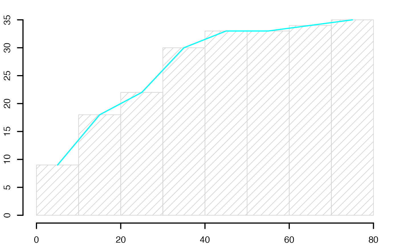
#axis(2,at=c(0,.2,.4,.6,.8,1)*length(data3),labels=c(0,.2,.4,.6,.8,1)*length(data3),lwd=2)
#suppressWarnings(par(oldpar))
pdf(file = paste(Chemin,"histopoleffcumnew",varN,".pdf",sep=""),
width = 8, height = 7, onefile = TRUE, family = "Helvetica",
title = "Histogramme des effectifs cumulés et polygone des effectifs cumulés", paper = "special", colormodel = colmodel)
par(mar = c(2, 2, 1, 1) + 0.1, mgp = c(2, 1, 0))
histoeffcum <- hist(data4,breaks=breaks0,main="",freq=T,xlab="",ylab="",lwd=2,density=10) #,yaxt="n"
segments(histoeffcum$mids[-(length(breaks0)-1)],histoeffcum$counts[-(length(breaks0)-1)],histoeffcum$mids[-1],histoeffcum$counts[-1],lwd=2,col="#00FFFF")
#axis(2,at=c(0,.2,.4,.6,.8,1)*length(data3),labels=c(0,.2,.4,.6,.8,1)*length(data3),lwd=2)
dev.off()
#> agg_png
#> 2Europe Salariés
data(Europe)
var1<- Europe$Salariés
varN <- "_Sal"
xi <- unique(sort(var1))
ni <- as.vector(table(var1))
data2 <- cbind(xi,ni)Diagramme en bâtons des effectifs
oldpar <- par()
par(mar = c(2, 2, 1, 1) + 0.1, mgp=c(2,1,0))
plot(xi,ni,type='h',xlab="",ylab="",lwd=2,ylim=c(0,max(ni))) #,xaxt="n"
#axis(1, at = 1:6, labels = c(1:5,6))
#axis(1, at = 1:6, labels = c(1:5,"6 et plus"))
#suppressWarnings(par(oldpar))
Chemin <- "~/Documents/Recherche/DeBoeck/Graphes/Donnees/"
colmodel="cmyk"
pdf(file = paste(Chemin,"batoneffnew",varN,".pdf",sep=""),
width = 8, height = 7, onefile = TRUE, family = "Helvetica",
title = "Diagramme en bâtons des effectifs", paper = "special", colormodel = colmodel)
par(mar = c(2, 2, 1, 1) + 0.1, mgp = c(2, 1, 0))
plot(xi,ni,type='h',xlab="",ylab="",lwd=2,ylim=c(0,max(ni))) #,xaxt="n"
dev.off()
#> agg_png
#> 2Diagramme en bâtons des effectifs et polygone des effectifs
oldpar <- par()
par(mar = c(2, 2, 1, 1) + 0.1, mgp=c(2,1,0))
plot(xi,ni/sum(ni),type='h',xlab="",ylab="",lwd=2,ylim=c(0,max(ni/sum(ni)))) #,xaxt="n"
#suppressWarnings(par(oldpar))
pdf(file = paste(Chemin,"batonfrenew",varN,".pdf",sep=""),
width = 8, height = 7, onefile = TRUE, family = "Helvetica",
title = "Probability or cumulative distribution graphs", paper = "special", colormodel = colmodel)
par(mar = c(2, 2, 1, 1) + 0.1, mgp = c(2, 1, 0))
plot(xi,ni/sum(ni),type='h',xlab="",ylab="",lwd=2,ylim=c(0,max(ni/sum(ni)))) #,xaxt="n"
dev.off()
#> agg_png
#> 2Diagramme en bâtons des effectifs et polygone des effectifs
oldpar <- par()
par(mar = c(2, 2, 1, 1) + 0.1, mgp=c(2,1,0))
plot(xi,ni,type='h',xlab="",ylab="",lwd=2,ylim=c(0,max(ni))) #,xaxt="n"
segments(xi[-length(xi)],ni[-length(xi)],xi[-1],ni[-1],lwd=2,col="#00FFFF")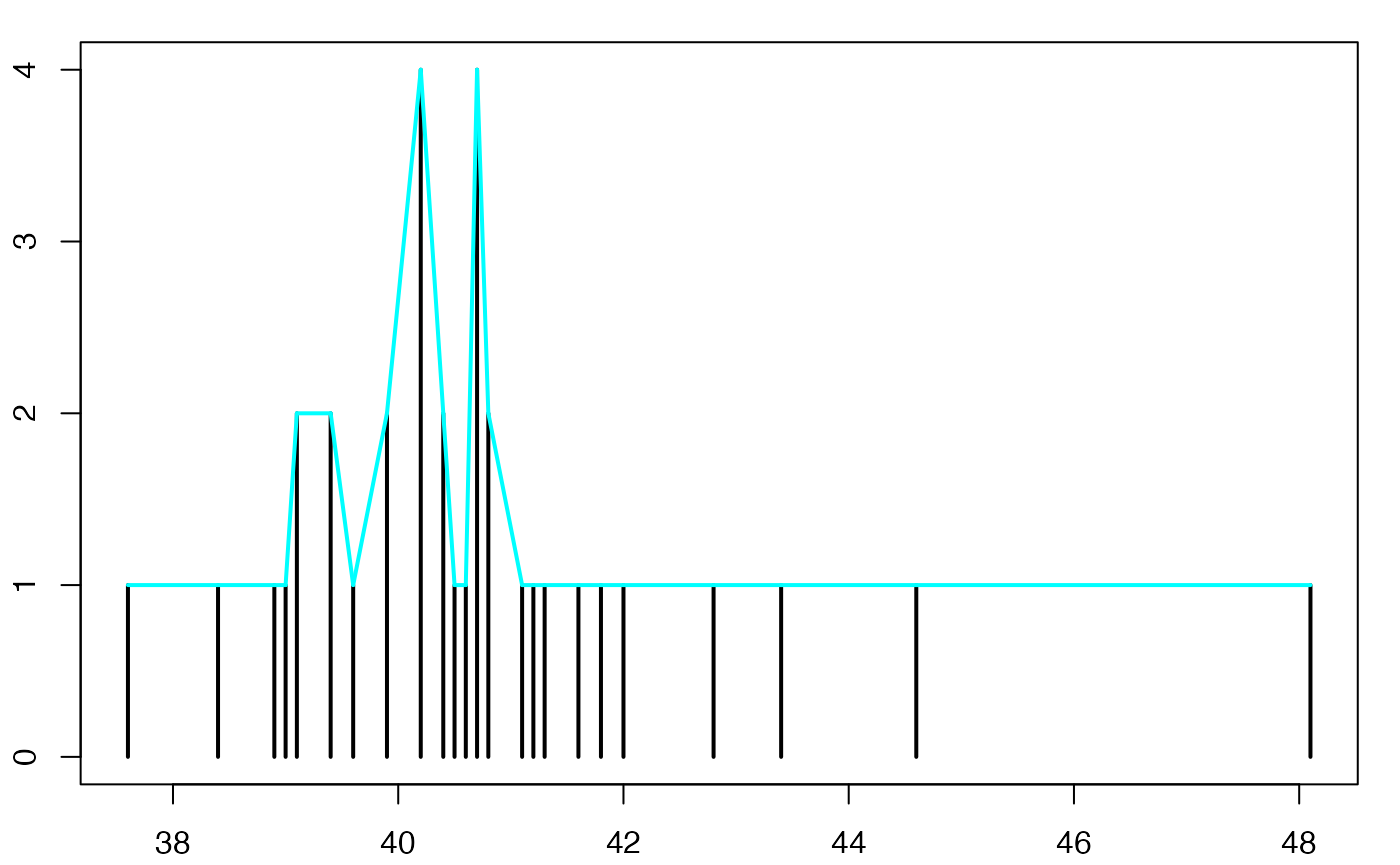
#suppressWarnings(par(oldpar))
pdf(file = paste(Chemin,"polyeffnew",varN,".pdf",sep=""),
width = 8, height = 7, onefile = TRUE, family = "Helvetica",
title = "Diagramme en bâtons des effectifs et polygone des effectifs", paper = "special", colormodel = colmodel)
par(mar = c(2, 2, 1, 1) + 0.1, mgp = c(2, 1, 0))
plot(xi,ni,type='h',xlab="",ylab="",lwd=2,ylim=c(0,max(ni))) #,xaxt="n"
segments(xi[-length(xi)],ni[-length(xi)],xi[-1],ni[-1],lwd=2,col="#00FFFF")
dev.off()
#> agg_png
#> 2Diagramme en bâtons des fréquences et polygone des fréquences
oldpar <- par()
par(mar = c(2, 2, 1, 1) + 0.1, mgp=c(2,1,0))
plot(xi,ni/sum(ni),type='h',xlab="",ylab="",lwd=2,ylim=c(0,max(ni/sum(ni))))
segments(xi[-length(xi)],ni[-length(xi)]/sum(ni),xi[-1],ni[-1]/sum(ni),lwd=2,col="#00FFFF")
#suppressWarnings(par(oldpar))
pdf(file = paste(Chemin,"polyfrenew",varN,".pdf",sep=""),
width = 8, height = 7, onefile = TRUE, family = "Helvetica",
title = "Diagramme en bâtons des fréquences et polygone des fréquences", paper = "special", colormodel = colmodel)
par(mar = c(2, 2, 1, 1) + 0.1, mgp = c(2, 1, 0))
plot(xi,ni/sum(ni),type='h',xlab="",ylab="",lwd=2,ylim=c(0,max(ni/sum(ni))))
segments(xi[-length(xi)],ni[-length(xi)]/sum(ni),xi[-1],ni[-1]/sum(ni),lwd=2,col="#00FFFF")
dev.off()
#> agg_png
#> 2Diagramme en bâtons des effectifs cumulés et polygone des effectifs cumulés
nisum <- rep(ni[1],length(ni))
for (iii in 2:length(ni))
{
nisum[iii] <- nisum[iii-1]+ni[iii]
}
oldpar <- par()
par(mar = c(2, 2, 1, 1) + 0.1, mgp=c(2,1,0))
plot(xi,nisum,type='h',xlab="",ylab="",lwd=2,ylim=c(0,max(nisum))) #,xaxt="n"
segments(xi[-length(xi)],nisum[-length(xi)],xi[-1],nisum[-1],lwd=2,col="#00FFFF")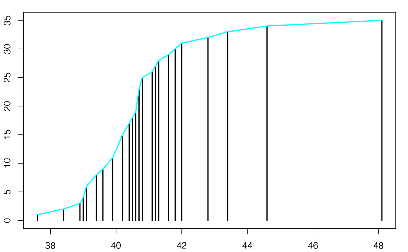
#suppressWarnings(par(oldpar))
pdf(file = paste(Chemin,"polyeffcumnew",varN,".pdf",sep=""),
width = 8, height = 7, onefile = TRUE, family = "Helvetica",
title = "Diagramme en bâtons des effectifs cumulés et polygone des effectifs cumulés", paper = "special", colormodel = colmodel)
par(mar = c(2, 2, 1, 1) + 0.1, mgp = c(2, 1, 0))
plot(xi,nisum,type='h',xlab="",ylab="",lwd=2,ylim=c(0,max(nisum))) #,xaxt="n"
segments(xi[-length(xi)],nisum[-length(xi)],xi[-1],nisum[-1],lwd=2,col="#00FFFF")
dev.off()
#> agg_png
#> 2Diagramme en bâtons des fréquences cumulées
oldpar <- par()
par(mar = c(2, 2, 1, 1) + 0.1, mgp=c(2,1,0))
plot(xi,nisum/sum(ni),type='h',xlab="",ylab="",lwd=2,ylim=c(0,max(nisum/sum(ni)))) #,xaxt="n"
#suppressWarnings(par(oldpar))
pdf(file = paste(Chemin,"frecumnew",varN,".pdf",sep=""),
width = 8, height = 7, onefile = TRUE, family = "Helvetica",
title = "Diagramme en bâtons des fréquences cumulées", paper = "special", colormodel = colmodel)
par(mar = c(2, 2, 1, 1) + 0.1, mgp = c(2, 1, 0))
plot(xi,nisum/sum(ni),type='h',xlab="",ylab="",lwd=2,ylim=c(0,max(nisum/sum(ni)))) #,xaxt="n"
dev.off()
#> agg_png
#> 2Diagramme en bâtons des effectifs cumulés
oldpar <- par()
par(mar = c(2, 2, 1, 1) + 0.1, mgp=c(2,1,0))
plot(xi,nisum,type='h',xlab="",ylab="",lwd=2,ylim=c(0,max(nisum))) #,xaxt="n"
#suppressWarnings(par(oldpar))
pdf(file = paste(Chemin,"effcumnew",varN,".pdf",sep=""),
width = 8, height = 7, onefile = TRUE, family = "Helvetica",
title = "Diagramme en bâtons des effectifs cumulés", paper = "special", colormodel = colmodel)
par(mar = c(2, 2, 1, 1) + 0.1, mgp = c(2, 1, 0))
plot(xi,nisum,type='h',xlab="",ylab="",lwd=2,ylim=c(0,max(nisum))) #,xaxt="n"
dev.off()
#> agg_png
#> 2Histogramme des fréquences
oldpar <- par()
par(mar = c(2, 2, 1, 1) + 0.1, mgp=c(2,1,0))
histofre <- hist(data3,breaks=breaks0,main="",freq=F,xlab="",ylab="",lwd=2,density=10)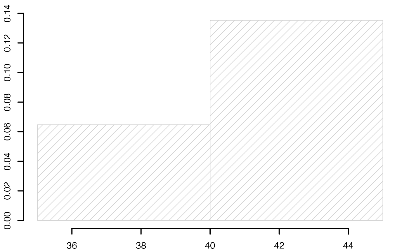
#suppressWarnings(par(oldpar))
Chemin <- "~/Documents/Recherche/DeBoeck/Graphes/Donnees/"
colmodel="cmyk"
pdf(file = paste(Chemin,"histofrenew",varN,".pdf",sep=""),
width = 8, height = 7, onefile = TRUE, family = "Helvetica",
title = "Histogramme des fréquences", paper = "special", colormodel = colmodel)
par(mar = c(2, 2, 1, 1) + 0.1, mgp = c(2, 1, 0))
histofre <- hist(data3,breaks=breaks0,main="",freq=F,xlab="",ylab="",lwd=2,density=10)
dev.off()
#> agg_png
#> 2Histogramme des fréquences et polygone des fréquences
oldpar <- par()
par(mar = c(2, 2, 1, 1) + 0.1, mgp=c(2,1,0))
histofre <- hist(data3,breaks=breaks0,main="",freq=F,xlab="",ylab="",lwd=2,density=10)
segments(histofre$mids[-(length(breaks0)-1)],histofre$density[-(length(breaks0)-1)],histofre$mids[-1],histofre$density[-1],lwd=2,col="#00FFFF")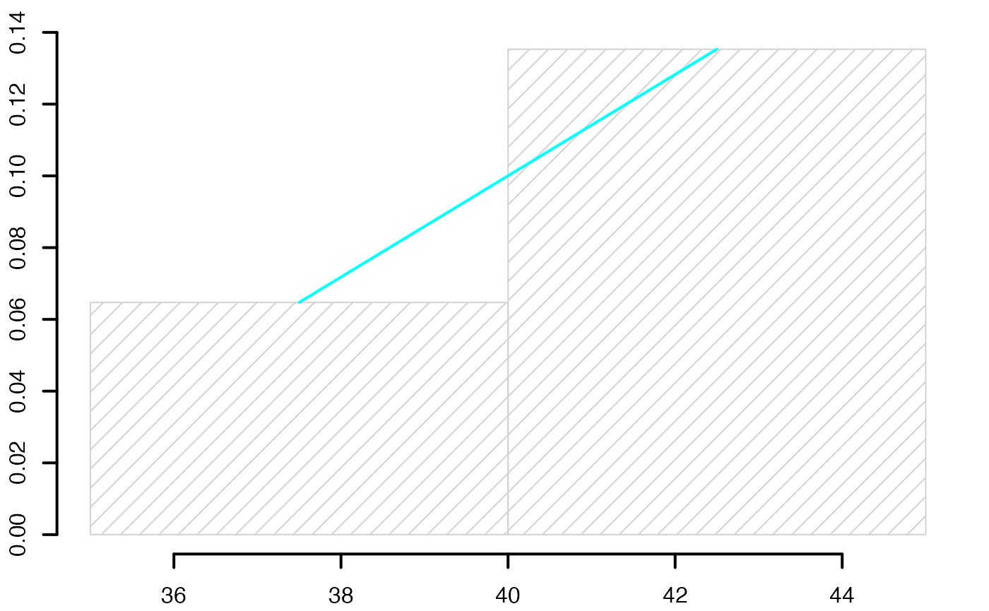
#suppressWarnings(par(oldpar))
pdf(file = paste(Chemin,"histopolfrenew",varN,".pdf",sep=""),
width = 8, height = 7, onefile = TRUE, family = "Helvetica",
title = "Histogramme des fréquences et polygone des fréquences", paper = "special", colormodel = colmodel)
par(mar = c(2, 2, 1, 1) + 0.1, mgp = c(2, 1, 0))
histofre <- hist(data3,breaks=breaks0,main="",freq=F,xlab="",ylab="",lwd=2,density=10)
segments(histofre$mids[-(length(breaks0)-1)],histofre$density[-(length(breaks0)-1)],histofre$mids[-1],histofre$density[-1],lwd=2,col="#00FFFF")
dev.off()
#> agg_png
#> 2Histogramme des fréquences cumulés
data4 <- rep((breaks0[-length(breaks0)]+diff(breaks0)/2)
,cumsum(table(cut(var1,breaks0))))
table(data4)
#> data4
#> 37.5 42.5
#> 11 34
oldpar <- par()
par(mar = c(2, 2, 1, 1) + 0.1, mgp=c(2,1,0))
histofrecum <- hist(data4,breaks=breaks0,main="",freq=F,xlab="",ylab="",lwd=2,yaxt="n",density=10)
axis(2,at=c(0,.2,.4,.6,.8,1)*max(histofrecum$dens),labels=c(0,.2,.4,.6,.8,1),lwd=2)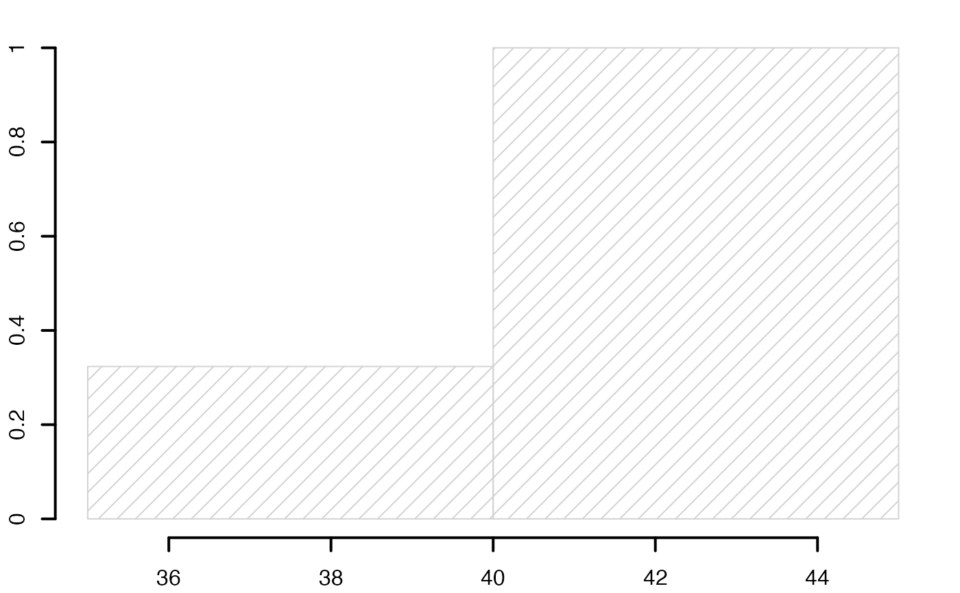
#suppressWarnings(par(oldpar))
pdf(file = paste(Chemin,"histofrecumnew",varN,".pdf",sep=""),
width = 8, height = 7, onefile = TRUE, family = "Helvetica",
title = "Histogramme des fréquences cumulés", paper = "special", colormodel = colmodel)
par(mar = c(2, 2, 1, 1) + 0.1, mgp = c(2, 1, 0))
histofrecum <- hist(data4,breaks=breaks0,main="",freq=F,xlab="",ylab="",lwd=2,yaxt="n",density=10)
axis(2,at=c(0,.2,.4,.6,.8,1)*max(histofrecum$dens),labels=c(0,.2,.4,.6,.8,1),lwd=2)
dev.off()
#> agg_png
#> 2Histogramme des fréquences cumulées et polygone des fréquences cumulées
oldpar <- par()
par(mar = c(2, 2, 1, 1) + 0.1, mgp=c(2,1,0))
histofrecum <- hist(data4,breaks=breaks0,main="",freq=F,xlab="",ylab="",lwd=2,yaxt="n",density=10)
segments(histofrecum$mids[-(length(breaks0)-1)],histofrecum$density[-(length(breaks0)-1)],histofrecum$mids[-1],histofrecum$density[-1],lwd=2,col="#00FFFF")
axis(2,at=c(0,.2,.4,.6,.8,1)*max(histofrecum$dens),labels=c(0,.2,.4,.6,.8,1),lwd=2)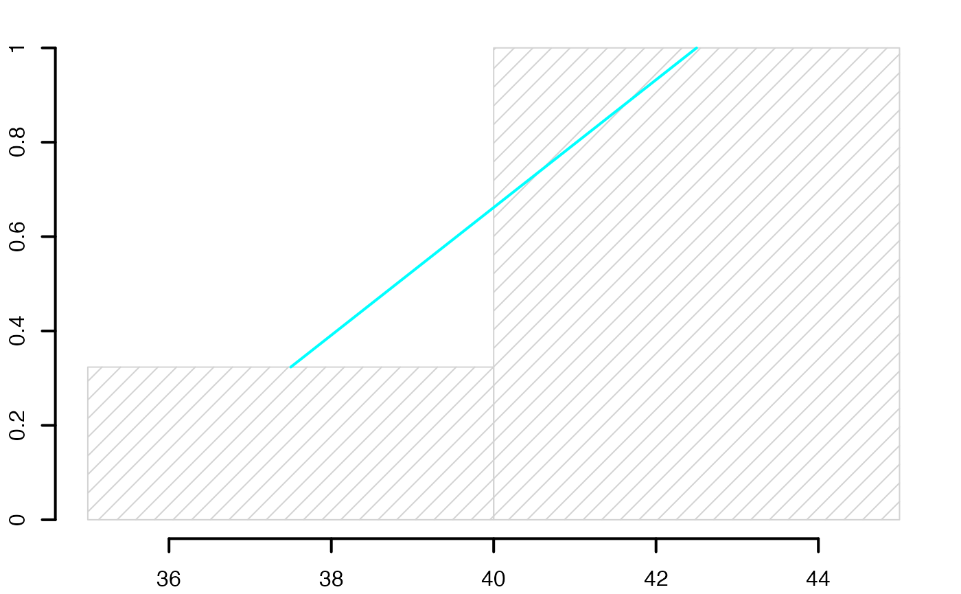
#suppressWarnings(par(oldpar))
pdf(file = paste(Chemin,"histopolfrecumnew",varN,".pdf",sep=""),
width = 8, height = 7, onefile = TRUE, family = "Helvetica",
title = "Histogramme des fréquences cumulées et polygone des fréquences cumulées", paper = "special", colormodel = colmodel)
par(mar = c(2, 2, 1, 1) + 0.1, mgp = c(2, 1, 0))
histofrecum <- hist(data4,breaks=breaks0,main="",freq=F,xlab="",ylab="",lwd=2,yaxt="n",density=10)
segments(histofrecum$mids[-(length(breaks0)-1)],histofrecum$density[-(length(breaks0)-1)],histofrecum$mids[-1],histofrecum$density[-1],lwd=2,col="#00FFFF")
axis(2,at=c(0,.2,.4,.6,.8,1)*max(histofrecum$dens),labels=c(0,.2,.4,.6,.8,1),lwd=2)
dev.off()
#> agg_png
#> 2Histogramme des effectifs cumulés et polygone des effectifs cumulés
oldpar <- par()
par(mar = c(2, 2, 1, 1) + 0.1, mgp=c(2,1,0))
histoeffcum <- hist(data4,breaks=breaks0,main="",freq=T,xlab="",ylab="",lwd=2,density=10) #,yaxt="n"
segments(histoeffcum$mids[-(length(breaks0)-1)],histoeffcum$counts[-(length(breaks0)-1)],histoeffcum$mids[-1],histoeffcum$counts[-1],lwd=2,col="#00FFFF")
#axis(2,at=c(0,.2,.4,.6,.8,1)*length(data3),labels=c(0,.2,.4,.6,.8,1)*length(data3),lwd=2)
#suppressWarnings(par(oldpar))
pdf(file = paste(Chemin,"histopoleffcumnew",varN,".pdf",sep=""),
width = 8, height = 7, onefile = TRUE, family = "Helvetica",
title = "Histogramme des effectifs cumulés et polygone des effectifs cumulés", paper = "special", colormodel = colmodel)
par(mar = c(2, 2, 1, 1) + 0.1, mgp = c(2, 1, 0))
histoeffcum <- hist(data4,breaks=breaks0,main="",freq=T,xlab="",ylab="",lwd=2,density=10) #,yaxt="n"
segments(histoeffcum$mids[-(length(breaks0)-1)],histoeffcum$counts[-(length(breaks0)-1)],histoeffcum$mids[-1],histoeffcum$counts[-1],lwd=2,col="#00FFFF")
#axis(2,at=c(0,.2,.4,.6,.8,1)*length(data3),labels=c(0,.2,.4,.6,.8,1)*length(data3),lwd=2)
dev.off()
#> agg_png
#> 2Europe Non-salariés
data(Europe)
var1<- Europe$NonSalariés
varN <- "_NonSal"
xi <- unique(sort(var1))
ni <- as.vector(table(var1))
data2 <- cbind(xi,ni)Diagramme en bâtons des effectifs
oldpar <- par()
par(mar = c(2, 2, 1, 1) + 0.1, mgp=c(2,1,0))
plot(xi,ni,type='h',xlab="",ylab="",lwd=2,ylim=c(0,max(ni))) #,xaxt="n"
#axis(1, at = 1:6, labels = c(1:5,6))
#axis(1, at = 1:6, labels = c(1:5,"6 et plus"))
#suppressWarnings(par(oldpar))
Chemin <- "~/Documents/Recherche/DeBoeck/Graphes/Donnees/"
colmodel="cmyk"
pdf(file = paste(Chemin,"batoneffnew",varN,".pdf",sep=""),
width = 8, height = 7, onefile = TRUE, family = "Helvetica",
title = "Diagramme en bâtons des effectifs", paper = "special", colormodel = colmodel)
par(mar = c(2, 2, 1, 1) + 0.1, mgp = c(2, 1, 0))
plot(xi,ni,type='h',xlab="",ylab="",lwd=2,ylim=c(0,max(ni))) #,xaxt="n"
dev.off()
#> agg_png
#> 2Diagramme en bâtons des fréquences
oldpar <- par()
par(mar = c(2, 2, 1, 1) + 0.1, mgp=c(2,1,0))
plot(xi,ni/sum(ni),type='h',xlab="",ylab="",lwd=2,ylim=c(0,max(ni/sum(ni)))) #,xaxt="n"
#suppressWarnings(par(oldpar))
pdf(file = paste(Chemin,"batonfrenew",varN,".pdf",sep=""),
width = 8, height = 7, onefile = TRUE, family = "Helvetica",
title = "Diagramme en bâtons des fréquences", paper = "special", colormodel = colmodel)
par(mar = c(2, 2, 1, 1) + 0.1, mgp = c(2, 1, 0))
plot(xi,ni/sum(ni),type='h',xlab="",ylab="",lwd=2,ylim=c(0,max(ni/sum(ni)))) #,xaxt="n"
dev.off()
#> agg_png
#> 2Diagramme en bâtons des effectifs et polygone des effectifs
oldpar <- par()
par(mar = c(2, 2, 1, 1) + 0.1, mgp=c(2,1,0))
plot(xi,ni,type='h',xlab="",ylab="",lwd=2,ylim=c(0,max(ni))) #,xaxt="n"
segments(xi[-length(xi)],ni[-length(xi)],xi[-1],ni[-1],lwd=2,col="#00FFFF")
#suppressWarnings(par(oldpar))
pdf(file = paste(Chemin,"polyeffnew",varN,".pdf",sep=""),
width = 8, height = 7, onefile = TRUE, family = "Helvetica",
title = "Diagramme en bâtons des effectifs et polygone des effectifs", paper = "special", colormodel = colmodel)
par(mar = c(2, 2, 1, 1) + 0.1, mgp = c(2, 1, 0))
plot(xi,ni,type='h',xlab="",ylab="",lwd=2,ylim=c(0,max(ni))) #,xaxt="n"
segments(xi[-length(xi)],ni[-length(xi)],xi[-1],ni[-1],lwd=2,col="#00FFFF")
dev.off()
#> agg_png
#> 2Diagramme en bâtons des fréquences et polygone des fréquences
oldpar <- par()
par(mar = c(2, 2, 1, 1) + 0.1, mgp=c(2,1,0))
plot(xi,ni/sum(ni),type='h',xlab="",ylab="",lwd=2,ylim=c(0,max(ni/sum(ni))))
segments(xi[-length(xi)],ni[-length(xi)]/sum(ni),xi[-1],ni[-1]/sum(ni),lwd=2,col="#00FFFF")
#suppressWarnings(par(oldpar))
pdf(file = paste(Chemin,"polyfrenew",varN,".pdf",sep=""),
width = 8, height = 7, onefile = TRUE, family = "Helvetica",
title = "Diagramme en bâtons des fréquences et polygone des fréquences", paper = "special", colormodel = colmodel)
par(mar = c(2, 2, 1, 1) + 0.1, mgp = c(2, 1, 0))
plot(xi,ni/sum(ni),type='h',xlab="",ylab="",lwd=2,ylim=c(0,max(ni/sum(ni))))
segments(xi[-length(xi)],ni[-length(xi)]/sum(ni),xi[-1],ni[-1]/sum(ni),lwd=2,col="#00FFFF")
dev.off()
#> agg_png
#> 2Diagramme en bâtons des effectifs cumulés et polygone des effectifs cumulés
nisum <- rep(ni[1],length(ni))
for (iii in 2:length(ni))
{
nisum[iii] <- nisum[iii-1]+ni[iii]
}
oldpar <- par()
par(mar = c(2, 2, 1, 1) + 0.1, mgp=c(2,1,0))
plot(xi,nisum,type='h',xlab="",ylab="",lwd=2,ylim=c(0,max(nisum))) #,xaxt="n"
segments(xi[-length(xi)],nisum[-length(xi)],xi[-1],nisum[-1],lwd=2,col="#00FFFF")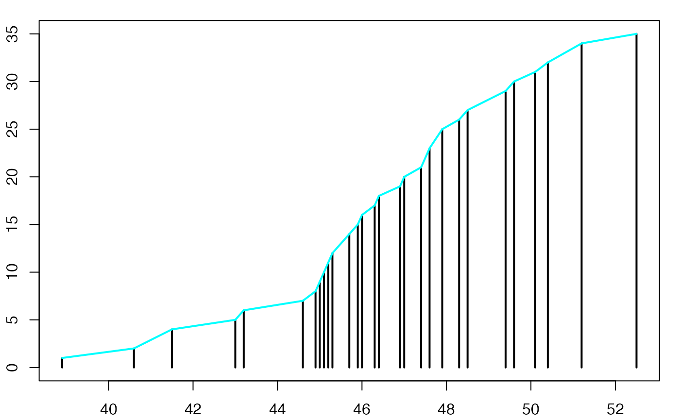
#suppressWarnings(par(oldpar))
pdf(file = paste(Chemin,"polyeffcumnew",varN,".pdf",sep=""),
width = 8, height = 7, onefile = TRUE, family = "Helvetica",
title = "Diagramme en bâtons des effectifs cumulés et polygone des effectifs cumulés", paper = "special", colormodel = colmodel)
par(mar = c(2, 2, 1, 1) + 0.1, mgp = c(2, 1, 0))
plot(xi,nisum,type='h',xlab="",ylab="",lwd=2,ylim=c(0,max(nisum))) #,xaxt="n"
segments(xi[-length(xi)],nisum[-length(xi)],xi[-1],nisum[-1],lwd=2,col="#00FFFF")
dev.off()
#> agg_png
#> 2Diagramme en bâtons des fréquences cumulées
oldpar <- par()
par(mar = c(2, 2, 1, 1) + 0.1, mgp=c(2,1,0))
plot(xi,nisum/sum(ni),type='h',xlab="",ylab="",lwd=2,ylim=c(0,max(nisum/sum(ni)))) #,xaxt="n"
#suppressWarnings(par(oldpar))
pdf(file = paste(Chemin,"frecumnew",varN,".pdf",sep=""),
width = 8, height = 7, onefile = TRUE, family = "Helvetica",
title = "Diagramme en bâtons des fréquences cumulées", paper = "special", colormodel = colmodel)
par(mar = c(2, 2, 1, 1) + 0.1, mgp = c(2, 1, 0))
plot(xi,nisum/sum(ni),type='h',xlab="",ylab="",lwd=2,ylim=c(0,max(nisum/sum(ni)))) #,xaxt="n"
dev.off()
#> agg_png
#> 2Diagramme en bâtons des effectifs cumulés
oldpar <- par()
par(mar = c(2, 2, 1, 1) + 0.1, mgp=c(2,1,0))
plot(xi,nisum,type='h',xlab="",ylab="",lwd=2,ylim=c(0,max(nisum))) #,xaxt="n"
#suppressWarnings(par(oldpar))
pdf(file = paste(Chemin,"effcumnew",varN,".pdf",sep=""),
width = 8, height = 7, onefile = TRUE, family = "Helvetica",
title = "Diagramme en bâtons des effectifs cumulés", paper = "special", colormodel = colmodel)
par(mar = c(2, 2, 1, 1) + 0.1, mgp = c(2, 1, 0))
plot(xi,nisum,type='h',xlab="",ylab="",lwd=2,ylim=c(0,max(nisum))) #,xaxt="n"
dev.off()
#> agg_png
#> 2Histogramme des fréquences
oldpar <- par()
par(mar = c(2, 2, 1, 1) + 0.1, mgp=c(2,1,0))
histofre <- hist(data3,breaks=breaks0,main="",freq=F,xlab="",ylab="",lwd=2,density=10)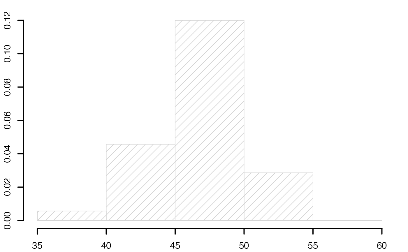
#suppressWarnings(par(oldpar))
Chemin <- "~/Documents/Recherche/DeBoeck/Graphes/Donnees/"
colmodel="cmyk"
pdf(file = paste(Chemin,"histofrenew",varN,".pdf",sep=""),
width = 8, height = 7, onefile = TRUE, family = "Helvetica",
title = "Histogramme des fréquences", paper = "special", colormodel = colmodel)
par(mar = c(2, 2, 1, 1) + 0.1, mgp = c(2, 1, 0))
histofre <- hist(data3,breaks=breaks0,main="",freq=F,xlab="",ylab="",lwd=2,density=10)
dev.off()
#> agg_png
#> 2Histogramme des fréquences et polygone des fréquences
oldpar <- par()
par(mar = c(2, 2, 1, 1) + 0.1, mgp=c(2,1,0))
histofre <- hist(data3,breaks=breaks0,main="",freq=F,xlab="",ylab="",lwd=2,density=10)
segments(histofre$mids[-(length(breaks0)-1)],histofre$density[-(length(breaks0)-1)],histofre$mids[-1],histofre$density[-1],lwd=2,col="#00FFFF")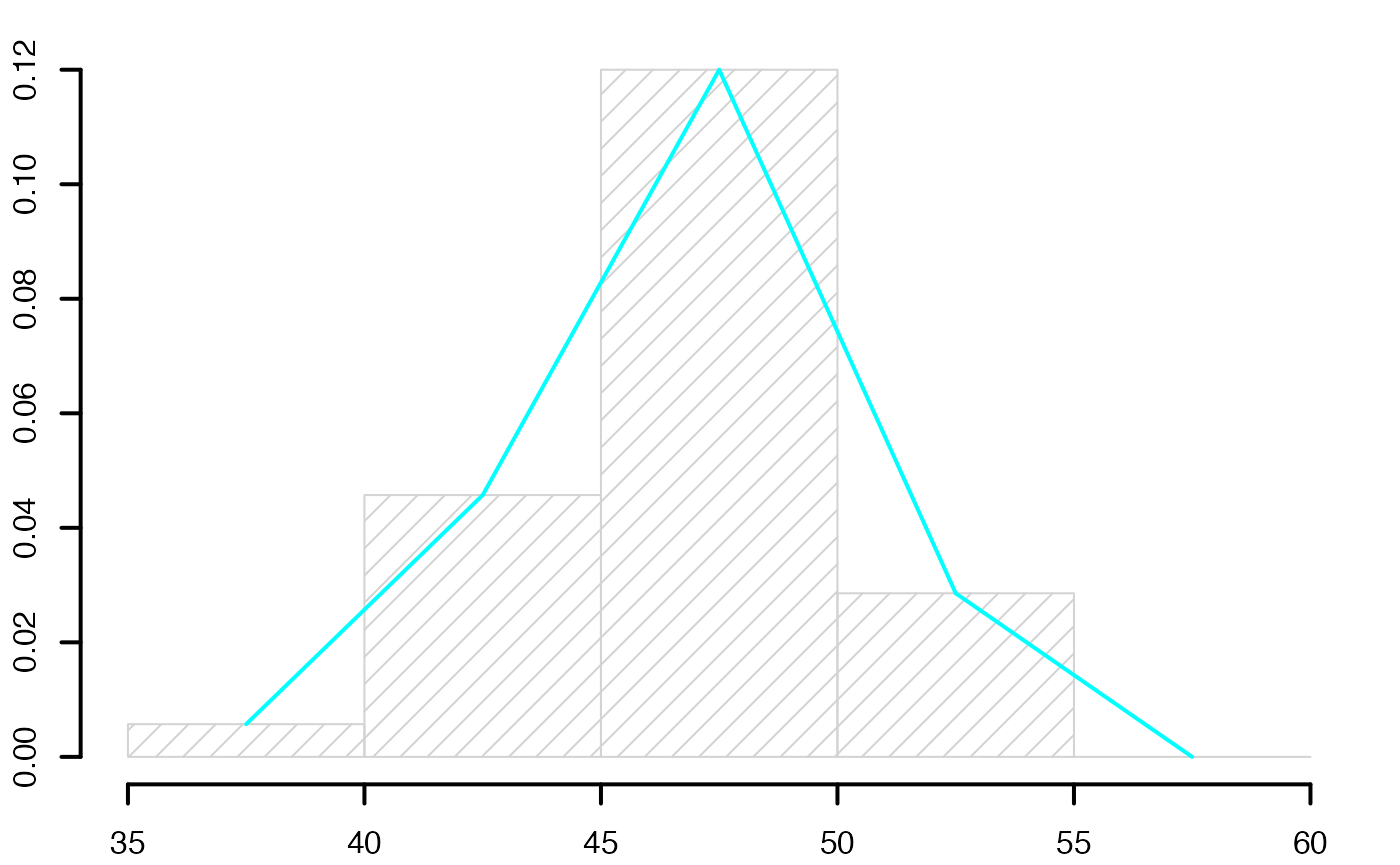
#suppressWarnings(par(oldpar))
pdf(file = paste(Chemin,"histopolfrenew",varN,".pdf",sep=""),
width = 8, height = 7, onefile = TRUE, family = "Helvetica",
title = "Histogramme des fréquences et polygone des fréquences", paper = "special", colormodel = colmodel)
par(mar = c(2, 2, 1, 1) + 0.1, mgp = c(2, 1, 0))
histofre <- hist(data3,breaks=breaks0,main="",freq=F,xlab="",ylab="",lwd=2,density=10)
segments(histofre$mids[-(length(breaks0)-1)],histofre$density[-(length(breaks0)-1)],histofre$mids[-1],histofre$density[-1],lwd=2,col="#00FFFF")
dev.off()
#> agg_png
#> 2Histogramme des effectifs cumulés et polygone des effectifs cumulés
oldpar <- par()
par(mar = c(2, 2, 1, 1) + 0.1, mgp=c(2,1,0))
histoeffcum <- hist(data4,breaks=breaks0,main="",freq=T,xlab="",ylab="",lwd=2,density=10) #,yaxt="n"
segments(histoeffcum$mids[-(length(breaks0)-1)],histoeffcum$counts[-(length(breaks0)-1)],histoeffcum$mids[-1],histoeffcum$counts[-1],lwd=2,col="#00FFFF")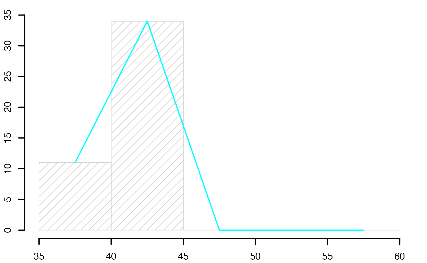
#axis(2,at=c(0,.2,.4,.6,.8,1)*length(data3),labels=c(0,.2,.4,.6,.8,1)*length(data3),lwd=2)
#suppressWarnings(par(oldpar))
pdf(file = paste(Chemin,"histopoleffcumnew",varN,".pdf",sep=""),
width = 8, height = 7, onefile = TRUE, family = "Helvetica",
title = "Histogramme des effectifs cumulés et polygone des effectifs cumulés", paper = "special", colormodel = colmodel)
par(mar = c(2, 2, 1, 1) + 0.1, mgp = c(2, 1, 0))
histoeffcum <- hist(data4,breaks=breaks0,main="",freq=T,xlab="",ylab="",lwd=2,density=10) #,yaxt="n"
segments(histoeffcum$mids[-(length(breaks0)-1)],histoeffcum$counts[-(length(breaks0)-1)],histoeffcum$mids[-1],histoeffcum$counts[-1],lwd=2,col="#00FFFF")
#axis(2,at=c(0,.2,.4,.6,.8,1)*length(data3),labels=c(0,.2,.4,.6,.8,1)*length(data3),lwd=2)
dev.off()
#> agg_png
#> 2Histogramme des fréquences cumulés
data4 <- rep((breaks0[-length(breaks0)]+diff(breaks0)/2)
,cumsum(table(cut(var1,breaks0))))
table(data4)
#> data4
#> 37.5 42.5 47.5 52.5 57.5
#> 1 9 30 35 35
oldpar <- par()
par(mar = c(2, 2, 1, 1) + 0.1, mgp=c(2,1,0))
histofrecum <- hist(data4,breaks=breaks0,main="",freq=F,xlab="",ylab="",lwd=2,yaxt="n",density=10)
axis(2,at=c(0,.2,.4,.6,.8,1)*max(histofrecum$dens),labels=c(0,.2,.4,.6,.8,1),lwd=2)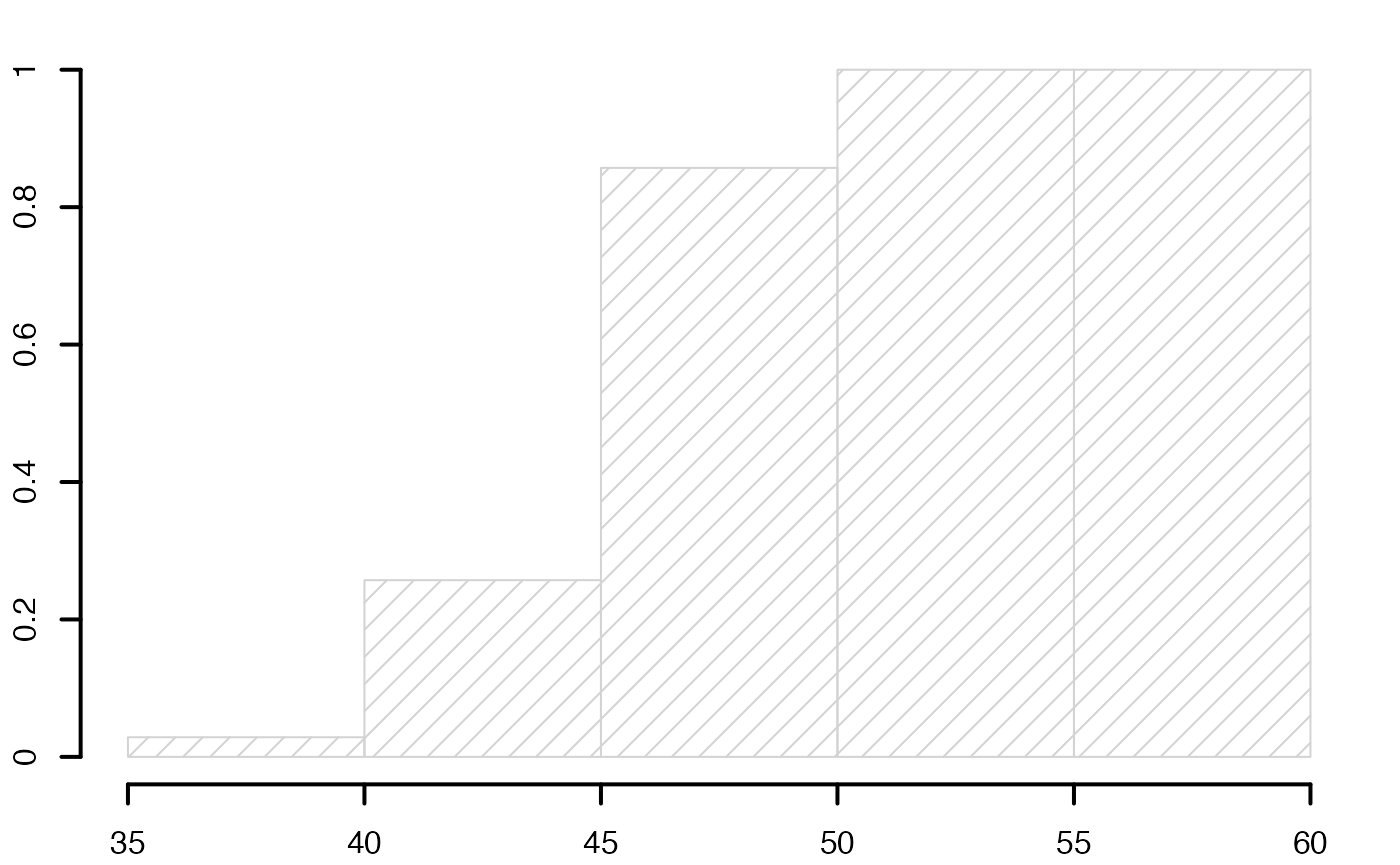
#suppressWarnings(par(oldpar))
pdf(file = paste(Chemin,"histofrecumnew",varN,".pdf",sep=""),
width = 8, height = 7, onefile = TRUE, family = "Helvetica",
title = "Histogramme des fréquences cumulés", paper = "special", colormodel = colmodel)
par(mar = c(2, 2, 1, 1) + 0.1, mgp = c(2, 1, 0))
histofrecum <- hist(data4,breaks=breaks0,main="",freq=F,xlab="",ylab="",lwd=2,yaxt="n",density=10)
axis(2,at=c(0,.2,.4,.6,.8,1)*max(histofrecum$dens),labels=c(0,.2,.4,.6,.8,1),lwd=2)
dev.off()
#> agg_png
#> 2Histogramme des fréquences cumulées et polygone des fréquences cumulées
oldpar <- par()
par(mar = c(2, 2, 1, 1) + 0.1, mgp=c(2,1,0))
histofrecum <- hist(data4,breaks=breaks0,main="",freq=F,xlab="",ylab="",lwd=2,yaxt="n",density=10)
segments(histofrecum$mids[-(length(breaks0)-1)],histofrecum$density[-(length(breaks0)-1)],histofrecum$mids[-1],histofrecum$density[-1],lwd=2,col="#00FFFF")
axis(2,at=c(0,.2,.4,.6,.8,1)*max(histofrecum$dens),labels=c(0,.2,.4,.6,.8,1),lwd=2)
#suppressWarnings(par(oldpar))
pdf(file = paste(Chemin,"histopolfrecumnew",varN,".pdf",sep=""),
width = 8, height = 7, onefile = TRUE, family = "Helvetica",
title = "Histogramme des fréquences cumulées et polygone des fréquences cumulées", paper = "special", colormodel = colmodel)
par(mar = c(2, 2, 1, 1) + 0.1, mgp = c(2, 1, 0))
histofrecum <- hist(data4,breaks=breaks0,main="",freq=F,xlab="",ylab="",lwd=2,yaxt="n",density=10)
segments(histofrecum$mids[-(length(breaks0)-1)],histofrecum$density[-(length(breaks0)-1)],histofrecum$mids[-1],histofrecum$density[-1],lwd=2,col="#00FFFF")
axis(2,at=c(0,.2,.4,.6,.8,1)*max(histofrecum$dens),labels=c(0,.2,.4,.6,.8,1),lwd=2)
dev.off()
#> agg_png
#> 2Histogramme des effectifs cumulés et polygone des effectifs cumulés
oldpar <- par()
par(mar = c(2, 2, 1, 1) + 0.1, mgp=c(2,1,0))
histoeffcum <- hist(data4,breaks=breaks0,main="",freq=T,xlab="",ylab="",lwd=2,density=10) #,yaxt="n"
segments(histoeffcum$mids[-(length(breaks0)-1)],histoeffcum$counts[-(length(breaks0)-1)],histoeffcum$mids[-1],histoeffcum$counts[-1],lwd=2,col="#00FFFF")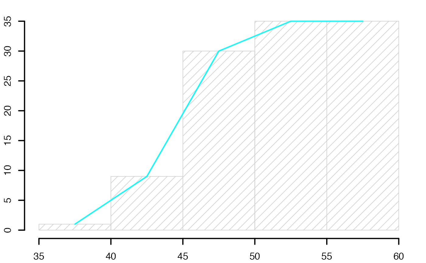
#axis(2,at=c(0,.2,.4,.6,.8,1)*length(data3),labels=c(0,.2,.4,.6,.8,1)*length(data3),lwd=2)
#suppressWarnings(par(oldpar))
pdf(file = paste(Chemin,"histopoleffcumnew",varN,".pdf",sep=""),
width = 8, height = 7, onefile = TRUE, family = "Helvetica",
title = "Histogramme des effectifs cumulés et polygone des effectifs cumulés", paper = "special", colormodel = colmodel)
par(mar = c(2, 2, 1, 1) + 0.1, mgp = c(2, 1, 0))
histoeffcum <- hist(data4,breaks=breaks0,main="",freq=T,xlab="",ylab="",lwd=2,density=10) #,yaxt="n"
segments(histoeffcum$mids[-(length(breaks0)-1)],histoeffcum$counts[-(length(breaks0)-1)],histoeffcum$mids[-1],histoeffcum$counts[-1],lwd=2,col="#00FFFF")
#axis(2,at=c(0,.2,.4,.6,.8,1)*length(data3),labels=c(0,.2,.4,.6,.8,1)*length(data3),lwd=2)
dev.off()
#> agg_png
#> 2Analyse du tableau Europe emploi
data(Europe)Paramètres de position
format(cbind(Moy=colMeans(Europe[,c(2,3,4,6,5)]), Q1=
c(quantile(Europe[,2],type=6)[2],quantile(Europe[,3],type=6)[2],quantile(Europe[,4],type=6)[2],quantile(Europe[,6],type=6)[2],quantile(Europe[,5],type=6)[2]), Q2=
c(quantile(Europe[,2],type=6)[3],quantile(Europe[,3],type=6)[3],quantile(Europe[,4],type=6)[3],quantile(Europe[,6],type=6)[3],quantile(Europe[,5],type=6)[3]), Q3=
c(quantile(Europe[,2],type=6)[4],quantile(Europe[,3],type=6)[4],quantile(Europe[,4],type=6)[4],quantile(Europe[,6],type=6)[4],quantile(Europe[,5],type=6)[4])),digits=3)
#> Moy Q1 Q2 Q3
#> Partiel_Ens "15.01" " 6.30" "11.30" "22.50"
#> Partiel_H " 8.03" " 4.70" " 6.60" "10.10"
#> Partiel_F "23.09" " 9.30" "17.00" "33.90"
#> NonSalariés "46.51" "45.00" "46.40" "48.50"
#> Salariés "40.72" "39.60" "40.50" "41.20"Paramètres de dispersion
tab2=cbind(
sd=c(sqrt(1/length(Europe[,2])*sum((Europe[,2]-mean(Europe[,2]))^2)),
sqrt(1/length(Europe[,3])*sum((Europe[,3]-mean(Europe[,3]))^2)),
sqrt(1/length(Europe[,4])*sum((Europe[,4]-mean(Europe[,4]))^2)),
sqrt(1/length(Europe[,6])*sum((Europe[,6]-mean(Europe[,6]))^2)),
sqrt(1/length(Europe[,5])*sum((Europe[,5]-mean(Europe[,5]))^2))
),
mad=c(quantile(abs(Europe[,2]-quantile(Europe[,2],type=6)[3]),type=6)[3],
quantile(abs(Europe[,3]-quantile(Europe[,3],type=6)[3]),type=6)[3],
quantile(abs(Europe[,4]-quantile(Europe[,4],type=6)[3]),type=6)[3],
quantile(abs(Europe[,6]-quantile(Europe[,6],type=6)[3]),type=6)[3],
quantile(abs(Europe[,5]-quantile(Europe[,5],type=6)[3]),type=6)[3]
),
Range=c(diff(range(Europe[,2])),
diff(range(Europe[,3])),
diff(range(Europe[,4])),
diff(range(Europe[,6])),
diff(range(Europe[,5])))
,
EIQ=c(quantile(Europe[,2],type=6)[4],quantile(Europe[,3],type=6)[4],quantile(Europe[,4],type=6)[4],quantile(Europe[,6],type=6)[4],quantile(Europe[,5],type=6)[4])-c(quantile(Europe[,2],type=6)[2],quantile(Europe[,3],type=6)[2],quantile(Europe[,4],type=6)[2],quantile(Europe[,6],type=6)[2],quantile(Europe[,5],type=6)[2])
,
CV=c(sqrt(1/length(Europe[,2])*sum((Europe[,2]-mean(Europe[,2]))^2)),
sqrt(1/length(Europe[,3])*sum((Europe[,3]-mean(Europe[,3]))^2)),
sqrt(1/length(Europe[,4])*sum((Europe[,4]-mean(Europe[,4]))^2)),
sqrt(1/length(Europe[,6])*sum((Europe[,6]-mean(Europe[,6]))^2)),
sqrt(1/length(Europe[,5])*sum((Europe[,5]-mean(Europe[,5]))^2)))/colMeans(Europe[,c(2,3,4,6,5)])*100)
rownames(tab2) <- colnames(Europe)[c(2,3,4,6,5)]
round(tab2,digits=3)
#> sd mad Range EIQ CV
#> Partiel_Ens 10.559 6.5 48.3 16.2 70.364
#> Partiel_H 5.071 2.9 26.2 5.4 63.184
#> Partiel_F 17.188 10.8 73.1 24.6 74.426
#> NonSalariés 3.074 1.5 13.6 3.5 6.610
#> Salariés 1.847 0.7 10.5 1.6 4.536Paramètres de forme
nn=length(Europe[,2])
tab5=
cbind(
AsyFis=
c(
1/nn*sum((Europe[,2]-mean(Europe[,2]))^3)/(1/nn*sum((Europe[,2]-mean(Europe[,2]))^2))^{3/2},
1/nn*sum((Europe[,3]-mean(Europe[,3]))^3)/(1/nn*sum((Europe[,3]-mean(Europe[,3]))^2))^{3/2},
1/nn*sum((Europe[,4]-mean(Europe[,4]))^3)/(1/nn*sum((Europe[,4]-mean(Europe[,4]))^2))^{3/2},
1/nn*sum((Europe[,5]-mean(Europe[,5]))^3)/(1/nn*sum((Europe[,5]-mean(Europe[,5]))^2))^{3/2},
1/nn*sum((Europe[,6]-mean(Europe[,6]))^3)/(1/nn*sum((Europe[,6]-mean(Europe[,6]))^2))^{3/2}
)
,
AsyPea=
c(
1/nn*sum((Europe[,2]-mean(Europe[,2]))^3)/(1/nn*sum((Europe[,2]-mean(Europe[,2]))^2))^{3/2},
1/nn*sum((Europe[,3]-mean(Europe[,3]))^3)/(1/nn*sum((Europe[,3]-mean(Europe[,3]))^2))^{3/2},
1/nn*sum((Europe[,4]-mean(Europe[,4]))^3)/(1/nn*sum((Europe[,4]-mean(Europe[,4]))^2))^{3/2},
1/nn*sum((Europe[,5]-mean(Europe[,5]))^3)/(1/nn*sum((Europe[,5]-mean(Europe[,5]))^2))^{3/2},
1/nn*sum((Europe[,6]-mean(Europe[,6]))^3)/(1/nn*sum((Europe[,6]-mean(Europe[,6]))^2))^{3/2}
)^2
,
AppFis=
c(
1/nn*sum((Europe[,2]-mean(Europe[,2]))^4)/(1/nn*sum((Europe[,2]-mean(Europe[,2]))^2))^{2},
1/nn*sum((Europe[,3]-mean(Europe[,3]))^4)/(1/nn*sum((Europe[,3]-mean(Europe[,3]))^2))^{2},
1/nn*sum((Europe[,4]-mean(Europe[,4]))^4)/(1/nn*sum((Europe[,4]-mean(Europe[,4]))^2))^{2},
1/nn*sum((Europe[,5]-mean(Europe[,5]))^4)/(1/nn*sum((Europe[,5]-mean(Europe[,5]))^2))^{2},
1/nn*sum((Europe[,6]-mean(Europe[,6]))^4)/(1/nn*sum((Europe[,6]-mean(Europe[,6]))^2))^{2}
)-3
,
AppPea=
c(
1/nn*sum((Europe[,2]-mean(Europe[,2]))^4)/(1/nn*sum((Europe[,2]-mean(Europe[,2]))^2))^{2},
1/nn*sum((Europe[,3]-mean(Europe[,3]))^4)/(1/nn*sum((Europe[,3]-mean(Europe[,3]))^2))^{2},
1/nn*sum((Europe[,4]-mean(Europe[,4]))^4)/(1/nn*sum((Europe[,4]-mean(Europe[,4]))^2))^{2},
1/nn*sum((Europe[,5]-mean(Europe[,5]))^4)/(1/nn*sum((Europe[,5]-mean(Europe[,5]))^2))^{2},
1/nn*sum((Europe[,6]-mean(Europe[,6]))^4)/(1/nn*sum((Europe[,6]-mean(Europe[,6]))^2))^{2}
)
)Analyse du tableau Europe emploi après regroupement des données
Création des groupes
Création naïve des classes
distg1<-table(cut(Europe$Partiel_Ens,c(0,10,20,30,40,50,60,70,80)))
distg2<-table(cut(Europe$Partiel_H,c(0,10,20,30,40,50,60,70,80)))
distg3<-table(cut(Europe$Partiel_F,c(0,10,20,30,40,50,60,70,80)))
distg1
#>
#> (0,10] (10,20] (20,30] (30,40] (40,50] (50,60] (60,70] (70,80]
#> 16 9 8 1 0 1 0 0
distg2
#>
#> (0,10] (10,20] (20,30] (30,40] (40,50] (50,60] (60,70] (70,80]
#> 25 9 1 0 0 0 0 0
distg3
#>
#> (0,10] (10,20] (20,30] (30,40] (40,50] (50,60] (60,70] (70,80]
#> 9 9 4 8 3 0 1 1
#Centres des classes
vald123<-(c(0,10,20,30,40,50,60,70,80)[-9]+c(0,10,20,30,40,50,60,70,80)[-1])/2
distg4<-table(cut(Europe$Salariés,c(35,40,45,50,55,60)))
distg5<-table(cut(Europe$NonSalariés,c(35,40,45,50,55,60)))
distg4
#>
#> (35,40] (40,45] (45,50] (50,55] (55,60]
#> 11 23 1 0 0
distg5
#>
#> (35,40] (40,45] (45,50] (50,55] (55,60]
#> 1 8 21 5 0
#Centres des classes
vald45<-(c(35,40,45,50,55,60)[-6]+c(35,40,45,50,55,60)[-1])/2Utilisation du package actuar
if(!("actuar" %in% installed.packages())){install.packages("actuar")}
library(actuar)
x1 <- grouped.data(Partiel_Ens=Europe$Partiel_Ens,breaks=c(0,10,20,30,40,50,60,70,80))
x2 <- grouped.data(Partiel_Ens=Europe$Partiel_H,breaks=c(0,10,20,30,40,50,60,70,80))
x3 <- grouped.data(Partiel_Ens=Europe$Partiel_F,breaks=c(0,10,20,30,40,50,60,70,80))
x4 <- grouped.data(Salariés=Europe$Salariés,breaks=c(0,10,20,30,40,50,60,70,80))
x5 <- grouped.data(NonSalariés=Europe$NonSalariés,breaks=c(0,10,20,30,40,50,60,70,80))
cbind(x1,x2,x3)
#> Var.1 Partiel_Ens Var.3 Partiel_Ens Var.5 Partiel_Ens
#> 1 (0, 10] 16 (0, 10] 25 (0, 10] 9
#> 2 (10, 20] 9 (10, 20] 9 (10, 20] 9
#> 3 (20, 30] 8 (20, 30] 1 (20, 30] 4
#> 4 (30, 40] 1 (30, 40] 0 (30, 40] 8
#> 5 (40, 50] 0 (40, 50] 0 (40, 50] 3
#> 6 (50, 60] 1 (50, 60] 0 (50, 60] 0
#> 7 (60, 70] 0 (60, 70] 0 (60, 70] 1
#> 8 (70, 80] 0 (70, 80] 0 (70, 80] 1
cbind(x4,x5)
#> Var.1 Salariés Var.3 NonSalariés
#> 1 (0, 10] 0 (0, 10] 0
#> 2 (10, 20] 0 (10, 20] 0
#> 3 (20, 30] 0 (20, 30] 0
#> 4 (30, 40] 11 (30, 40] 1
#> 5 (40, 50] 24 (40, 50] 29
#> 6 (50, 60] 0 (50, 60] 5
#> 7 (60, 70] 0 (60, 70] 0
#> 8 (70, 80] 0 (70, 80] 0Statistiques descriptives groupées
c(
weighted.mean(vald123,distg1),
weighted.mean(vald123,distg2),
weighted.mean(vald123,distg2),
weighted.mean(vald45,distg4),
weighted.mean(vald45,distg5)
)
#> [1] 14.428571 8.142857 8.142857 41.071429 46.785714
tab3=cbind(
c(
mean(x1),
mean(x2),
mean(x3),
mean(x4),
mean(x5)
),
rbind(quantile(x1),quantile(x2),quantile(x3),quantile(x4),quantile(x5))[,c(2,3,4)]
)
round(c(
mean(x1),
mean(x2),
mean(x3),
mean(x4),
mean(x5)
),digits=2)
#> Partiel_Ens Partiel_Ens Partiel_Ens Salariés NonSalariés
#> 14.43 8.14 23.86 41.86 46.14
round( rbind(quantile(x1),quantile(x2),quantile(x3),quantile(x4),quantile(x5))[,c(2,3,4)],digits=2)
#> 25% 50% 75%
#> [1,] 5.47 11.67 21.56
#> [2,] 3.50 7.00 11.39
#> [3,] 9.72 19.44 35.31
#> [4,] 37.95 42.71 46.35
#> [5,] 42.67 45.69 48.71
round(tab3,digits=2)
#> 25% 50% 75%
#> Partiel_Ens 14.43 5.47 11.67 21.56
#> Partiel_Ens 8.14 3.50 7.00 11.39
#> Partiel_Ens 23.86 9.72 19.44 35.31
#> Salariés 41.86 37.95 42.71 46.35
#> NonSalariés 46.14 42.67 45.69 48.71
tab4=cbind(
sigma=c(
sqrt(weighted.mean(((x1[,1][-1]+x1[,1][-length(x1[,1])])/2-mean(x1))^2,x1[,2])-1/12*weighted.mean(diff(x1[,1])^2,x1[,2])),
sqrt(weighted.mean(((x2[,1][-1]+x2[,1][-length(x2[,1])])/2-mean(x2))^2,x2[,2])-1/12*weighted.mean(diff(x2[,1])^2,x2[,2])),
sqrt(weighted.mean(((x3[,1][-1]+x3[,1][-length(x3[,1])])/2-mean(x3))^2,x3[,2])-1/12*weighted.mean(diff(x3[,1])^2,x3[,2])),
sqrt(weighted.mean(((x4[,1][-1]+x4[,1][-length(x4[,1])])/2-mean(x4))^2,x4[,2])-1/12*weighted.mean(diff(x4[,1])^2,x4[,2])),
sqrt(weighted.mean(((x5[,1][-1]+x5[,1][-length(x5[,1])])/2-mean(x5))^2,x5[,2])-1/12*weighted.mean(diff(x5[,1])^2,x5[,2]))
),
EIQ=t(diff(t(rbind(quantile(x1),quantile(x2),quantile(x3),quantile(x4),quantile(x5))[,c(2,4)]))),
CV=c(
sqrt(weighted.mean(((x1[,1][-1]+x1[,1][-length(x1[,1])])/2-mean(x1))^2,x1[,2])-1/12*weighted.mean(diff(x1[,1])^2,x1[,2]))/mean(x1)*100,
sqrt(weighted.mean(((x2[,1][-1]+x2[,1][-length(x2[,1])])/2-mean(x2))^2,x2[,2])-1/12*weighted.mean(diff(x2[,1])^2,x2[,2]))/mean(x2)*100,
sqrt(weighted.mean(((x3[,1][-1]+x3[,1][-length(x3[,1])])/2-mean(x3))^2,x3[,2])-1/12*weighted.mean(diff(x3[,1])^2,x3[,2]))/mean(x3)*100,
sqrt(weighted.mean(((x4[,1][-1]+x4[,1][-length(x4[,1])])/2-mean(x4))^2,x4[,2])-1/12*weighted.mean(diff(x4[,1])^2,x4[,2]))/mean(x4)*100,
sqrt(weighted.mean(((x5[,1][-1]+x5[,1][-length(x5[,1])])/2-mean(x5))^2,x5[,2])-1/12*weighted.mean(diff(x5[,1])^2,x5[,2]))/mean(x5)*100
))
round(tab4[,1],digits=2)
#> Partiel_Ens Partiel_Ens Partiel_Ens Salariés NonSalariés
#> 10.82 4.35 17.12 3.64 2.74
round(tab4[,2],digits=2)
#> Partiel_Ens Partiel_Ens Partiel_Ens Salariés NonSalariés
#> 16.09 7.89 25.59 8.40 6.03
round(tab4[,3],digits=2)
#> Partiel_Ens Partiel_Ens Partiel_Ens Salariés NonSalariés
#> 74.98 53.43 71.78 8.69 5.94
tab6=cbind(
asyFis=
c(
weighted.mean(((x1[,1][-1]+x1[,1][-length(x1[,1])])/2-mean(x1))^3,x1[,2])/sqrt(weighted.mean(((x1[,1][-1]+x1[,1][-length(x1[,1])])/2-mean(x1))^2,x1[,2])-1/12*weighted.mean(diff(x1[,1])^2,x1[,2]))^3,
weighted.mean(((x2[,1][-1]+x2[,1][-length(x2[,1])])/2-mean(x2))^3,x2[,2])/sqrt(weighted.mean(((x2[,1][-1]+x2[,1][-length(x2[,1])])/2-mean(x2))^2,x2[,2])-1/12*weighted.mean(diff(x2[,1])^2,x2[,2]))^3,
weighted.mean(((x3[,1][-1]+x3[,1][-length(x3[,1])])/2-mean(x3))^3,x3[,2])/sqrt(weighted.mean(((x3[,1][-1]+x3[,1][-length(x3[,1])])/2-mean(x3))^2,x3[,2])-1/12*weighted.mean(diff(x3[,1])^2,x3[,2]))^3,
weighted.mean(((x4[,1][-1]+x4[,1][-length(x4[,1])])/2-mean(x4))^3,x4[,2])/sqrt(weighted.mean(((x4[,1][-1]+x4[,1][-length(x4[,1])])/2-mean(x4))^2,x4[,2])-1/12*weighted.mean(diff(x4[,1])^2,x4[,2]))^3,
weighted.mean(((x5[,1][-1]+x5[,1][-length(x5[,1])])/2-mean(x5))^3,x5[,2])/sqrt(weighted.mean(((x5[,1][-1]+x5[,1][-length(x5[,1])])/2-mean(x5))^2,x5[,2])-1/12*weighted.mean(diff(x5[,1])^2,x5[,2]))^3
)
,
asyPea=
c(
weighted.mean(((x1[,1][-1]+x1[,1][-length(x1[,1])])/2-mean(x1))^3,x1[,2])/sqrt(weighted.mean(((x1[,1][-1]+x1[,1][-length(x1[,1])])/2-mean(x1))^2,x1[,2])-1/12*weighted.mean(diff(x1[,1])^2,x1[,2]))^3,
weighted.mean(((x2[,1][-1]+x2[,1][-length(x2[,1])])/2-mean(x2))^3,x2[,2])/sqrt(weighted.mean(((x2[,1][-1]+x2[,1][-length(x2[,1])])/2-mean(x2))^2,x2[,2])-1/12*weighted.mean(diff(x2[,1])^2,x2[,2]))^3,
weighted.mean(((x3[,1][-1]+x3[,1][-length(x3[,1])])/2-mean(x3))^3,x3[,2])/sqrt(weighted.mean(((x3[,1][-1]+x3[,1][-length(x3[,1])])/2-mean(x3))^2,x3[,2])-1/12*weighted.mean(diff(x3[,1])^2,x3[,2]))^3,
weighted.mean(((x4[,1][-1]+x4[,1][-length(x4[,1])])/2-mean(x4))^3,x4[,2])/sqrt(weighted.mean(((x4[,1][-1]+x4[,1][-length(x4[,1])])/2-mean(x4))^2,x4[,2])-1/12*weighted.mean(diff(x4[,1])^2,x4[,2]))^3,
weighted.mean(((x5[,1][-1]+x5[,1][-length(x5[,1])])/2-mean(x5))^3,x5[,2])/sqrt(weighted.mean(((x5[,1][-1]+x5[,1][-length(x5[,1])])/2-mean(x5))^2,x5[,2])-1/12*weighted.mean(diff(x5[,1])^2,x5[,2]))^3
)^2
,
appFis=
c(
(weighted.mean(((x1[,1][-1]+x1[,1][-length(x1[,1])])/2-mean(x1))^4,x1[,2])
-10^2/2*weighted.mean(((x1[,1][-1]+x1[,1][-length(x1[,1])])/2-mean(x1))^2,x1[,2])
+7/240*10^4)/sqrt(weighted.mean(((x1[,1][-1]+x1[,1][-length(x1[,1])])/2-mean(x1))^2,x1[,2])-1/12*weighted.mean(diff(x1[,1])^2,x1[,2]))^4,
(weighted.mean(((x2[,1][-1]+x2[,1][-length(x2[,1])])/2-mean(x2))^4,x2[,2])
-10^2/2*weighted.mean(((x2[,1][-1]+x2[,1][-length(x2[,1])])/2-mean(x2))^2,x2[,2])
+7/240*10^4)/sqrt(weighted.mean(((x2[,1][-1]+x2[,1][-length(x2[,1])])/2-mean(x2))^2,x2[,2])-1/12*weighted.mean(diff(x2[,1])^2,x2[,2]))^4,
(weighted.mean(((x3[,1][-1]+x3[,1][-length(x3[,1])])/2-mean(x3))^4,x3[,2])
-10^2/2*weighted.mean(((x3[,1][-1]+x3[,1][-length(x3[,1])])/2-mean(x3))^2,x3[,2])
+7/240*10^4)/sqrt(weighted.mean(((x3[,1][-1]+x3[,1][-length(x3[,1])])/2-mean(x3))^2,x3[,2])-1/12*weighted.mean(diff(x3[,1])^2,x3[,2]))^4,
(weighted.mean(((x4[,1][-1]+x4[,1][-length(x4[,1])])/2-mean(x4))^4,x4[,2])
-10^2/2*weighted.mean(((x4[,1][-1]+x4[,1][-length(x4[,1])])/2-mean(x4))^2,x4[,2])
+7/240*10^4)/sqrt(weighted.mean(((x4[,1][-1]+x4[,1][-length(x4[,1])])/2-mean(x4))^2,x4[,2])-1/12*weighted.mean(diff(x4[,1])^2,x4[,2]))^4,
(weighted.mean(((x5[,1][-1]+x5[,1][-length(x5[,1])])/2-mean(x5))^4,x5[,2])
-10^2/2*weighted.mean(((x5[,1][-1]+x5[,1][-length(x5[,1])])/2-mean(x5))^2,x5[,2])
+7/240*10^4)/sqrt(weighted.mean(((x5[,1][-1]+x5[,1][-length(x5[,1])])/2-mean(x5))^2,x5[,2])-1/12*weighted.mean(diff(x5[,1])^2,x5[,2]))^4
)-3
,
appPea=
c(
(weighted.mean(((x1[,1][-1]+x1[,1][-length(x1[,1])])/2-mean(x1))^4,x1[,2])
-10^2/2*weighted.mean(((x1[,1][-1]+x1[,1][-length(x1[,1])])/2-mean(x1))^2,x1[,2])
+7/240*10^4)/sqrt(weighted.mean(((x1[,1][-1]+x1[,1][-length(x1[,1])])/2-mean(x1))^2,x1[,2])-1/12*weighted.mean(diff(x1[,1])^2,x1[,2]))^4,
(weighted.mean(((x2[,1][-1]+x2[,1][-length(x2[,1])])/2-mean(x2))^4,x2[,2])
-10^2/2*weighted.mean(((x2[,1][-1]+x2[,1][-length(x2[,1])])/2-mean(x2))^2,x2[,2])
+7/240*10^4)/sqrt(weighted.mean(((x2[,1][-1]+x2[,1][-length(x2[,1])])/2-mean(x2))^2,x2[,2])-1/12*weighted.mean(diff(x2[,1])^2,x2[,2]))^4,
(weighted.mean(((x3[,1][-1]+x3[,1][-length(x3[,1])])/2-mean(x3))^4,x3[,2])
-10^2/2*weighted.mean(((x3[,1][-1]+x3[,1][-length(x3[,1])])/2-mean(x3))^2,x3[,2])
+7/240*10^4)/sqrt(weighted.mean(((x3[,1][-1]+x3[,1][-length(x3[,1])])/2-mean(x3))^2,x3[,2])-1/12*weighted.mean(diff(x3[,1])^2,x3[,2]))^4,
(weighted.mean(((x4[,1][-1]+x4[,1][-length(x4[,1])])/2-mean(x4))^4,x4[,2])
-10^2/2*weighted.mean(((x4[,1][-1]+x4[,1][-length(x4[,1])])/2-mean(x4))^2,x4[,2])
+7/240*10^4)/sqrt(weighted.mean(((x4[,1][-1]+x4[,1][-length(x4[,1])])/2-mean(x4))^2,x4[,2])-1/12*weighted.mean(diff(x4[,1])^2,x4[,2]))^4,
(weighted.mean(((x5[,1][-1]+x5[,1][-length(x5[,1])])/2-mean(x5))^4,x5[,2])
-10^2/2*weighted.mean(((x5[,1][-1]+x5[,1][-length(x5[,1])])/2-mean(x5))^2,x5[,2])
+7/240*10^4)/sqrt(weighted.mean(((x5[,1][-1]+x5[,1][-length(x5[,1])])/2-mean(x5))^2,x5[,2])-1/12*weighted.mean(diff(x5[,1])^2,x5[,2]))^4
)
)
rownames(tab6) <- colnames(Europe[,-1])
round(tab6,digits=2)
#> asyFis asyPea appFis appPea
#> Partiel_Ens 1.61 2.60 3.06 6.06
#> Partiel_H 2.40 5.75 2.23 5.23
#> Partiel_F 1.00 1.01 0.69 3.69
#> Salariés -1.67 2.77 -3.14 -0.14
#> NonSalariés 2.85 8.10 11.58 14.58