Chapitre 08. Théorie des probabilités.

Tout le code avec R.

F. Bertrand et M. Maumy

2025-09-22

if(!("sageR" %in% installed.packages())){install.packages("sageR")}
library(sageR)

Exemple de fonction de probabilité et de fonction de répartition d’une v.a. discrète finie

if(!("spatstat" %in% installed.packages())){install.packages("spatstat")}
library(spatstat)
if(!("ggplot2" %in% installed.packages())){install.packages("ggplot2")}
library(ggplot2)
source("https://raw.githubusercontent.com/NicolasWoloszko/stat_ecdf_weighted/master/stat_ecdf_weighted.R")

xp <- data.frame(cbind(x=c(1,7/3,4,13/2),p=c(1/6,1/6,1/6,1/2),sp=c(1/6,1/3,1/2,1)))
ggplot(aes(x=x),data = xp)  + geom_point(aes(y=sp),data = xp,col="#00FFFF") + geom_bar(aes(y=p), width=.025, stat="identity") + xlim(0,8) + ylab("Probabilité") + stat_ecdf(aes(x=x,weight=p),geom = "step",col="#00FFFF", lty=2)+ geom_point(aes(y=p),data = xp)+ annotate("text", x = .5, y = .95,
  label = paste(expression(p[X])),
  parse=TRUE) + annotate("text", x = .5, y = .875,
  label = paste(expression(F[X])),
  parse=TRUE,col="#00FFFF") +  geom_segment(aes(x = 0, y = .95, xend = .3, yend = .95), data = xp)  +  geom_segment(aes(x = 0, y = .90, xend = .3, yend = .90), data = xp, col="#00FFFF", lty=2) 
#> Warning in stat_ecdf(aes(x = x, weight = p), geom = "step", col = "#00FFFF", :
#> Ignoring unknown aesthetics: weight
#> Warning in geom_segment(aes(x = 0, y = 0.95, xend = 0.3, yend = 0.95), data = xp): All aesthetics have length 1, but the data has 4 rows.
#> ℹ Please consider using `annotate()` or provide this layer with data containing
#>   a single row.
#> Warning in geom_segment(aes(x = 0, y = 0.9, xend = 0.3, yend = 0.9), data = xp, : All aesthetics have length 1, but the data has 4 rows.
#> ℹ Please consider using `annotate()` or provide this layer with data containing
#>   a single row.
#> Warning: The following aesthetics were dropped during statistical transformation:
#> weight.
#> ℹ This can happen when ggplot fails to infer the correct grouping structure in
#>   the data.
#> ℹ Did you forget to specify a `group` aesthetic or to convert a numerical
#>   variable into a factor?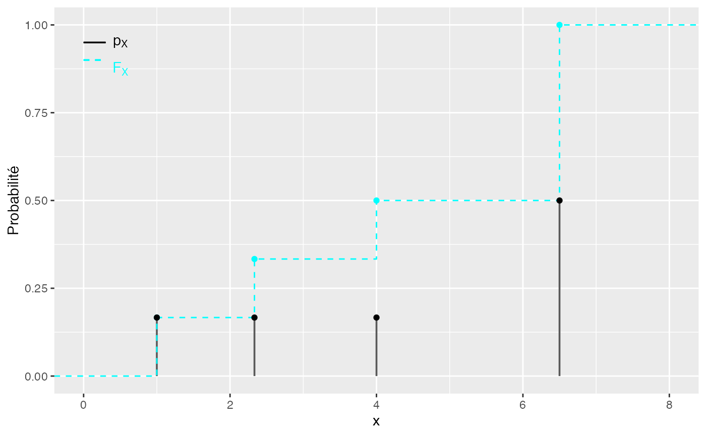

Chemin = "~/Documents/Recherche/DeBoeck/Graphes/Fichiers/"
colmodel="cmyk"
ggsave(filename = paste(Chemin,"exemple_probas.pdf",sep=""),
       width = 12, height = 8, onefile = TRUE, family = "Helvetica",
    title = "Probability or cumulative distribution graphs", paper = "special", colormodel = colmodel)

ggsave(filename = paste(Chemin,"exemple_probas_2.pdf",sep=""),
       width = 6, height = 4, onefile = TRUE, family = "Helvetica",
    title = "Probability or cumulative distribution graphs", paper = "special", colormodel = colmodel)

Exemple de fonction de densité de probabilité et de fonction de répartition d’une v.a. continue

Fonction de densité de probabilité

library(ggplot2)
densx = function(x) return((x>=0)*(x<=1)*2*x)
ggplot() + xlim(-.5, 1.5) + ylim(0, 2) + geom_function(fun = densx, n=10^4, lwd=1)+ ylab("Densité de probabilité")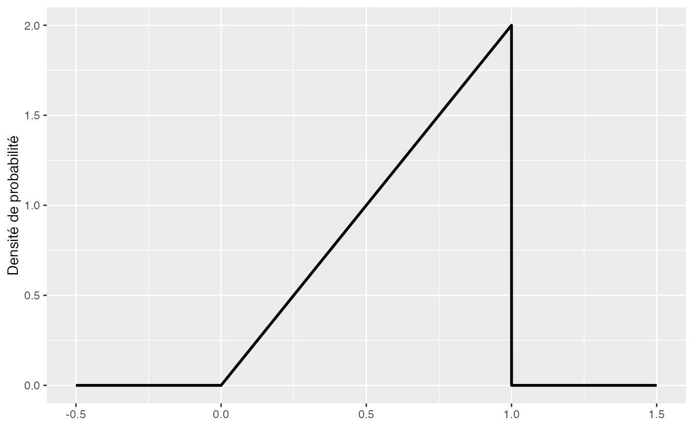

Chemin = "~/Documents/Recherche/DeBoeck/Graphes/Fichiers/"
colmodel="cmyk"
ggsave(filename = paste(Chemin,"exemple_probas_dens_cont.pdf",sep=""),
       width = 12, height = 8, onefile = TRUE, family = "Helvetica",
    title = "Probability or cumulative distribution graphs", paper = "special", colormodel = colmodel)

ggsave(filename = paste(Chemin,"exemple_probas_dens_cont_2.pdf",sep=""),
       width = 6, height = 4, onefile = TRUE, family = "Helvetica",
    title = "Probability or cumulative distribution graphs", paper = "special", colormodel = colmodel)

Fonction de densité de répartition

library(ggplot2)
Frepx = function(x) return((x>=0)*(x<=1)*x^2+(x>=1))
ggplot() + xlim(-.5, 1.5) + ylim(0, 1) + geom_function(fun = Frepx, n=10^4, lwd=1)+ ylab("Probabilité cumulée")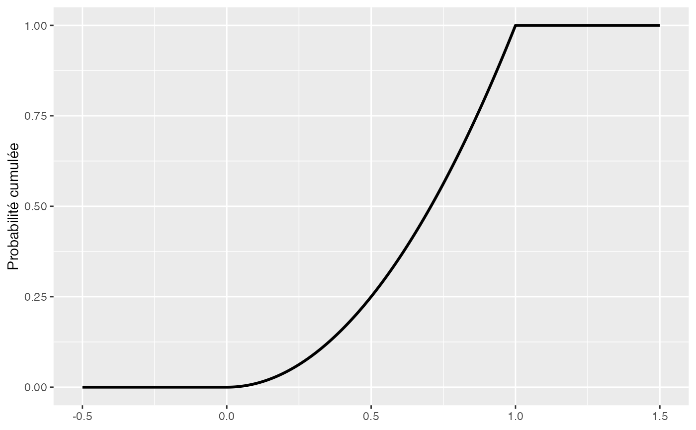

Chemin = "~/Documents/Recherche/DeBoeck/Graphes/Fichiers/"
colmodel="cmyk"
ggsave(filename = paste(Chemin,"exemple_probas_frep_cont.pdf",sep=""),
       width = 12, height = 8, onefile = TRUE, family = "Helvetica",
    title = "Probability or cumulative distribution graphs", paper = "special", colormodel = colmodel)

ggsave(filename = paste(Chemin,"exemple_probas_frep_cont_2.pdf",sep=""),
       width = 6, height = 4, onefile = TRUE, family = "Helvetica",
    title = "Probability or cumulative distribution graphs", paper = "special", colormodel = colmodel)

Représentations graphiques de lois discrètes

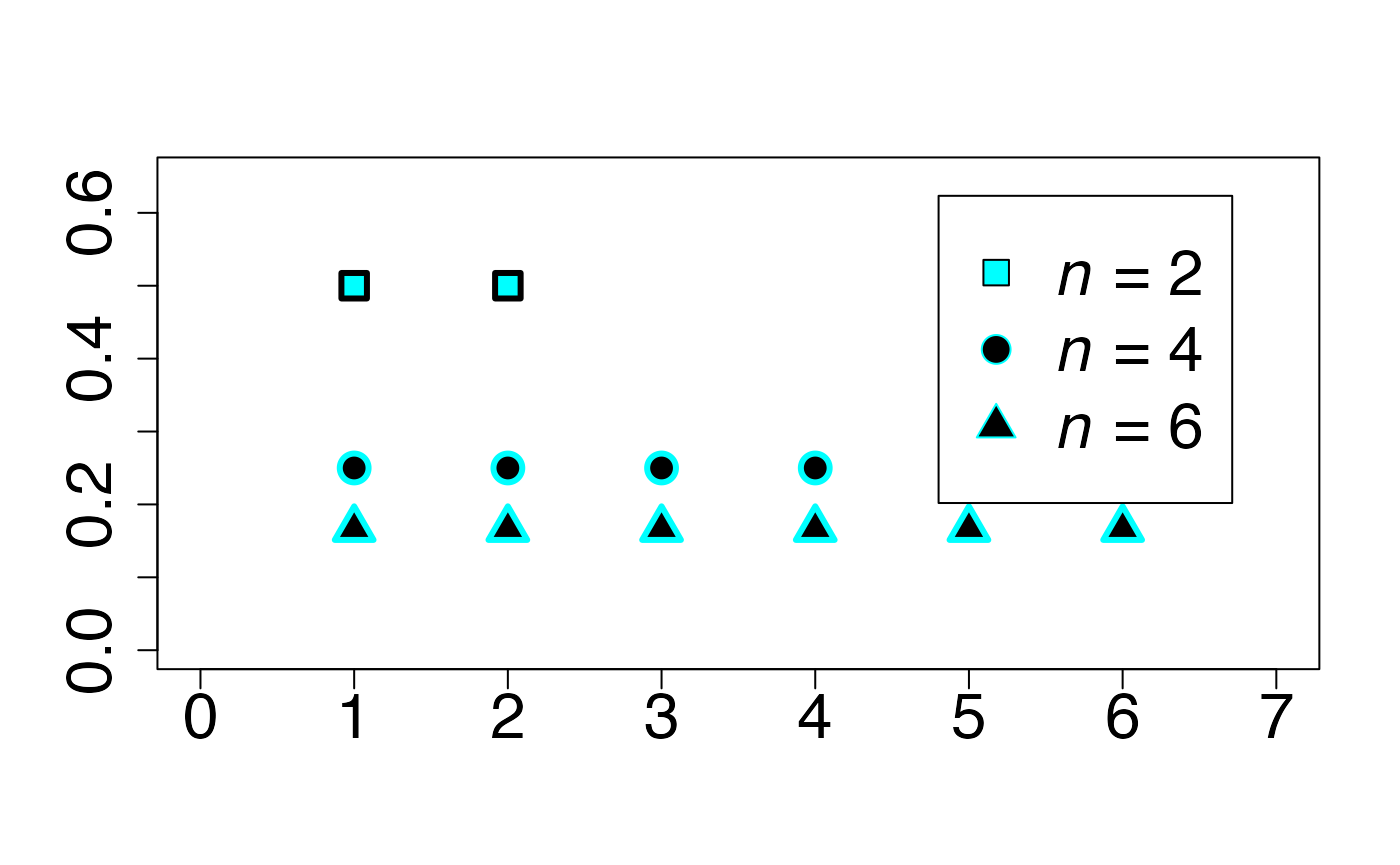
Loi uniforme discrète

Chemin = "~/Documents/Recherche/DeBoeck/Graphes/Fichiers/"
colmodel="cmyk"
pdf(file = paste(Chemin,"dens_",LOI,".pdf",sep=""),
    width = 8, height = 7, onefile = TRUE, family = "Helvetica",
    title = "Probability or cumulative distribution graphs", paper = "special", colormodel = colmodel)
infx=0;supx=7;
infy=0;supy=0.65;
ddiscunif <- function(x,N) (if(sum(x == 1:N)) {1/N} else {0})
fd <- function(x) {ddiscunif(x,2)}
plot(cbind(1:2,sapply(1:2,fd)),xlim=c(infx,supx),ylim=c(infy,supy),type="p",ylab="",xlab="",pch=22,bg=bgmagentas[1],cex=2,lwd=3,col=colmagentas[1],cex.axis=2)
fd <- function(x) {ddiscunif(x,4)}
points(cbind(1:4,sapply(1:4,fd)),xlim=c(infx,supx),ylim=c(infy,supy),type="p",ylab="",xlab="",pch=21,bg=bgmagentas[2],cex=2,lwd=3,col=colmagentas[2],new=T)
fd <- function(x) {ddiscunif(x,6)}
points(cbind(1:6,sapply(1:6,fd)),xlim=c(infx,supx),ylim=c(infy,supy),type="p",ylab="",xlab="",pch=24,bg=bgmagentas[3],cex=2,lwd=3,col=colmagentas[3],new=T)
leg.txt <- c(expression(paste(italic(n)," = 2",sep="")), expression(paste(italic(n)," = 4",sep="")),
             expression(paste(italic(n)," = 6",sep="")))
legend("topright", leg.txt, pch = c(22, 21, 24), col = c(colmagentas[1],colmagentas[2],colmagentas[3]), pt.bg = c(bgmagentas[1],bgmagentas[2],bgmagentas[3]), cex = 2, bg="white", inset=.075)# , pch = "*"
dev.off()
#> agg_png 
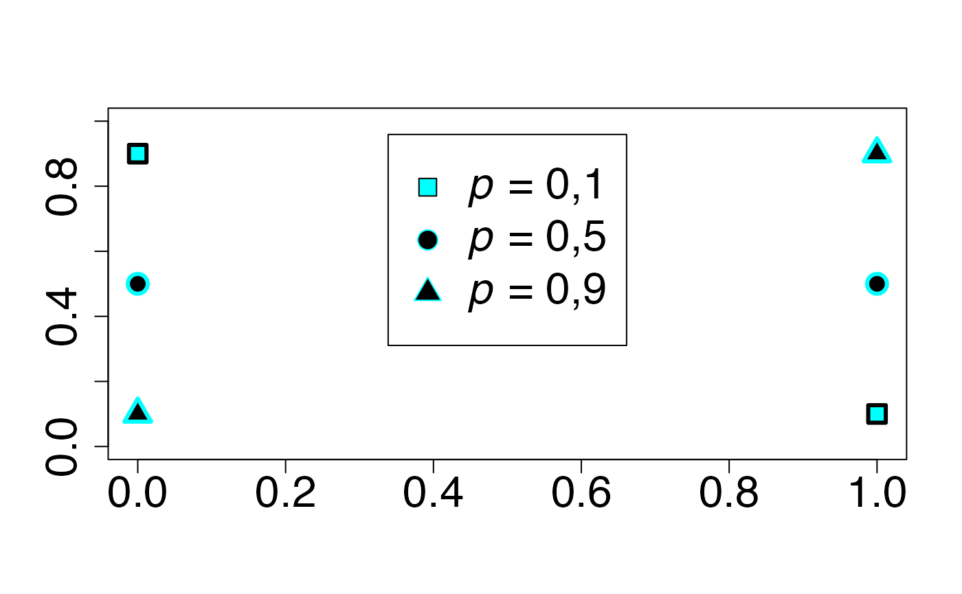
#>       2

Loi de Bernoulli

Chemin = "~/Documents/Recherche/DeBoeck/Graphes/Fichiers/"
colmodel="cmyk"
pdf(file = paste(Chemin,"dens_",LOI,".pdf",sep=""),
    width = 8, height = 7, onefile = TRUE, family = "Helvetica",
    title = "Probability or cumulative distribution graphs", paper = "special", colormodel = colmodel)
infx=0;supx=1;
infy=0;supy=1;
fd <- function(x) {dbinom(x,1,0.1)}
plot(cbind(0:5,sapply(0:5,fd)),xlim=c(infx,supx),ylim=c(infy,supy),type="p",ylab="",xlab="",pch=22,bg=bgmagentas[1],cex=2,lwd=3,col=colmagentas[1],cex.axis=2)
fd <- function(x) {dbinom(x,1,0.5)}
points(cbind(0:10,sapply(0:10,fd)),xlim=c(infx,supx),ylim=c(infy,supy),type="p",ylab="",xlab="",pch=21,bg=bgmagentas[2],cex=2,lwd=3,col=colmagentas[2],new=T)
fd <- function(x) {dbinom(x,1,0.9)}
points(cbind(0:20,sapply(0:20,fd)),xlim=c(infx,supx),ylim=c(infy,supy),type="p",ylab="",xlab="",pch=24,bg=bgmagentas[3],cex=2,lwd=3,col=colmagentas[3],new=T)
leg.txt <- c(expression(paste(italic(p)," = 0,1",sep="")), expression(paste(italic(p)," = 0,5",sep="")),
             expression(paste(italic(p)," = 0,9",sep="")))
legend("top", leg.txt, pch = c(22, 21, 24), col = c(colmagentas[1],colmagentas[2],colmagentas[3]), pt.bg = c(bgmagentas[1],bgmagentas[2],bgmagentas[3]), cex = 2, bg="white", inset=.075)# , pch = "*"
dev.off()
#> agg_png 
#>       2

Loi binomiale (cas symétrique)

#> agg_png 
#>       2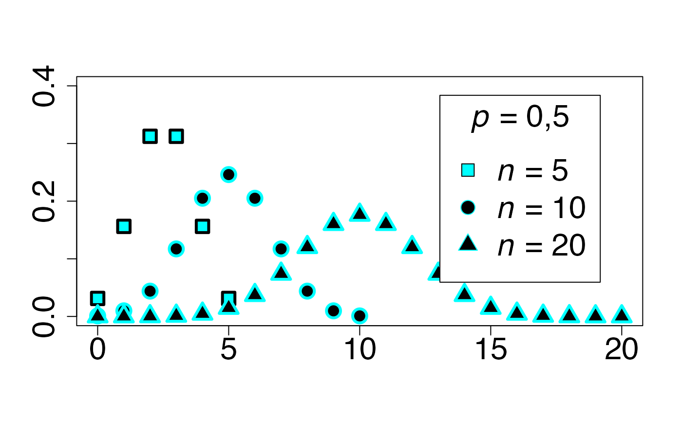

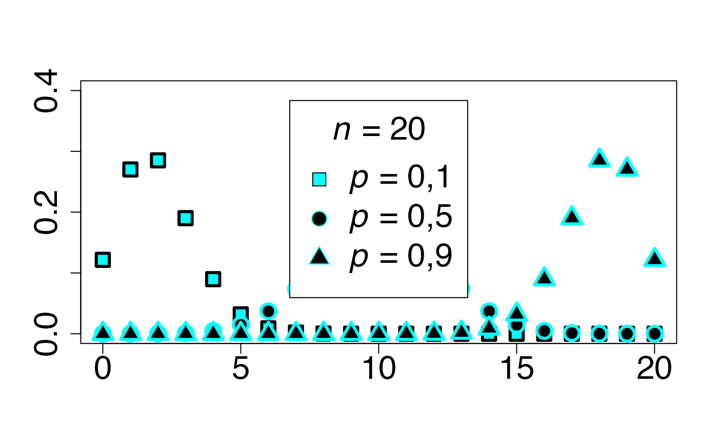
Loi binomiale (cas asymétrique)

Chemin = "~/Documents/Recherche/DeBoeck/Graphes/Fichiers/"
colmodel="cmyk"
pdf(file = paste(Chemin,"dens_",LOI,".pdf",sep=""),
    width = 8, height = 7, onefile = TRUE, family = "Helvetica",
    title = "Probability or cumulative distribution graphs", paper = "special", colormodel = colmodel)
infx=0;supx=20;
infy=0;supy=0.40;
fd <- function(x) {dbinom(x,20,0.1)}
plot(cbind(0:20,sapply(0:20,fd)),xlim=c(infx,supx),ylim=c(infy,supy),type="p",ylab="",xlab="",pch=22,bg=bgmagentas[1],cex=2,lwd=3,col=colmagentas[1],cex.axis=2)
fd <- function(x) {dbinom(x,20,0.5)}
points(cbind(0:20,sapply(0:20,fd)),xlim=c(infx,supx),ylim=c(infy,supy),type="p",ylab="",xlab="",pch=21,bg=bgmagentas[2],cex=2,lwd=3,col=colmagentas[2],new=T)
fd <- function(x) {dbinom(x,20,0.9)}
points(cbind(0:20,sapply(0:20,fd)),xlim=c(infx,supx),ylim=c(infy,supy),type="p",ylab="",xlab="",pch=24,bg=bgmagentas[3],cex=2,lwd=3,col=colmagentas[3],new=T)
leg.txt <- c(expression(paste(italic(p)," = 0,1",sep="")), expression(paste(italic(p)," = 0,5",sep="")),
             expression(paste(italic(p)," = 0,9",sep="")))
legend("top", leg.txt, title = expression(paste(italic(n)," = 20",sep="")) , pch = c(22, 21, 24), col = c(colmagentas[1],colmagentas[2],colmagentas[3]), pt.bg = c(bgmagentas[1],bgmagentas[2],bgmagentas[3]), cex = 2, bg="white", inset=.075)# , pch = "*"
dev.off()
#> agg_png 
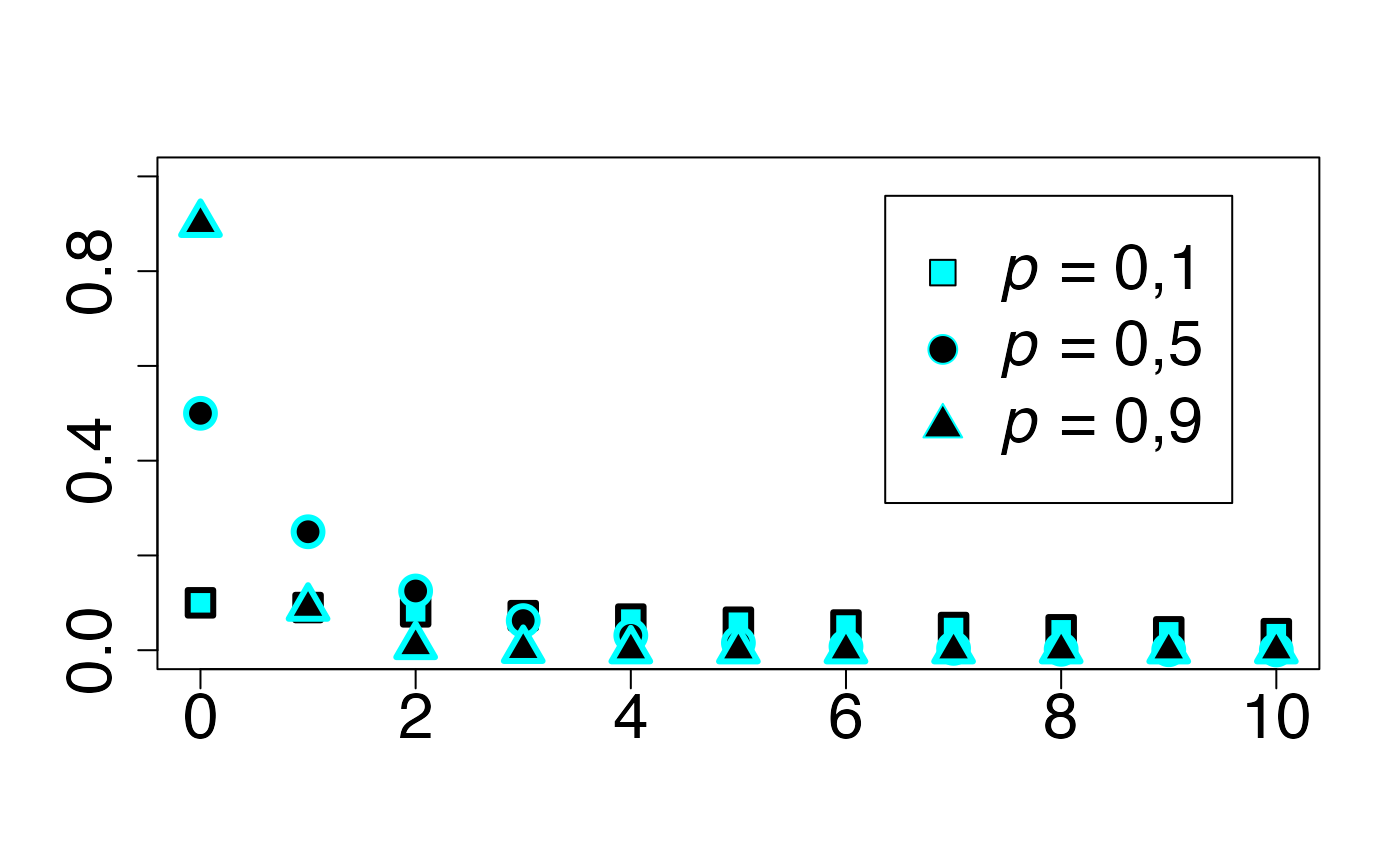
#>       2

Loi géométrique

Chemin = "~/Documents/Recherche/DeBoeck/Graphes/Fichiers/"
colmodel="cmyk"
pdf(file = paste(Chemin,"dens_",LOI,".pdf",sep=""),
    width = 8, height = 7, onefile = TRUE, family = "Helvetica",
    title = "Probability or cumulative distribution graphs", paper = "special", colormodel = colmodel)
infx=0;supx=10;
infy=0;supy=1;
fd <- function(x) {dgeom(x,0.1)}
plot(cbind(0:20,sapply(0:20,fd)),xlim=c(infx,supx),ylim=c(infy,supy),type="p",ylab="",xlab="",pch=22,bg=bgmagentas[1],cex=2,lwd=3,col=colmagentas[1],cex.axis=2)
fd <- function(x) {dgeom(x,0.5)}
points(cbind(0:20,sapply(0:20,fd)),xlim=c(infx,supx),ylim=c(infy,supy),type="p",ylab="",xlab="",pch=21,bg=bgmagentas[2],cex=2,lwd=3,col=colmagentas[2],new=T)
fd <- function(x) {dgeom(x,0.9)}
points(cbind(0:20,sapply(0:20,fd)),xlim=c(infx,supx),ylim=c(infy,supy),type="p",ylab="",xlab="",pch=24,bg=bgmagentas[3],cex=2,lwd=3,col=colmagentas[3],new=T)
leg.txt <- c(expression(paste(italic(p)," = 0,1",sep="")), expression(paste(italic(p)," = 0,5",sep="")),
             expression(paste(italic(p)," = 0,9",sep="")))
legend("topright", leg.txt, pch = c(22, 21, 24), col = c(colmagentas[1],colmagentas[2],colmagentas[3]), pt.bg = c(bgmagentas[1],bgmagentas[2],bgmagentas[3]), cex = 2, bg="white", inset=.075)# , pch = "*"
dev.off()
#> agg_png 
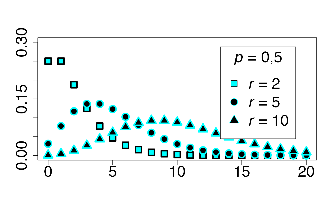
#>       2

Loi négative binomiale (cas symétrique)

Chemin = "~/Documents/Recherche/DeBoeck/Graphes/Fichiers/"
colmodel="cmyk"
pdf(file = paste(Chemin,"dens_",LOI,".pdf",sep=""),
    width = 8, height = 7, onefile = TRUE, family = "Helvetica",
    title = "Probability or cumulative distribution graphs", paper = "special", colormodel = colmodel)
infx=0;supx=20;
infy=0;supy=0.30;
fd <- function(x) {dnbinom(x,2,0.5)}
plot(cbind(0:20,sapply(0:20,fd)),xlim=c(infx,supx),ylim=c(infy,supy),type="p",ylab="",xlab="",pch=22,bg=bgmagentas[1],cex=2,lwd=3,col=colmagentas[1],cex.axis=2)
fd <- function(x) {dnbinom(x,5,0.5)}
points(cbind(0:20,sapply(0:20,fd)),xlim=c(infx,supx),ylim=c(infy,supy),type="p",ylab="",xlab="",pch=21,bg=bgmagentas[2],cex=2,lwd=3,col=colmagentas[2],new=T)
fd <- function(x) {dnbinom(x,10,0.5)}
points(cbind(0:20,sapply(0:20,fd)),xlim=c(infx,supx),ylim=c(infy,supy),type="p",ylab="",xlab="",pch=24,bg=bgmagentas[3],cex=2,lwd=3,col=colmagentas[3],new=T)
leg.txt <- c(expression(paste(italic(r)," = 2",sep="")), expression(paste(italic(r)," = 5",sep="")),
             expression(paste(italic(r)," = 10",sep="")))
legend("topright", leg.txt, title = expression(paste(italic(p)," = 0,5",sep="")) , pch = c(22, 21, 24), col = c(colmagentas[1],colmagentas[2],colmagentas[3]), pt.bg = c(bgmagentas[1],bgmagentas[2],bgmagentas[3]), cex = 2, bg="white", inset=.075)# , pch = "*"
dev.off()
#> agg_png 
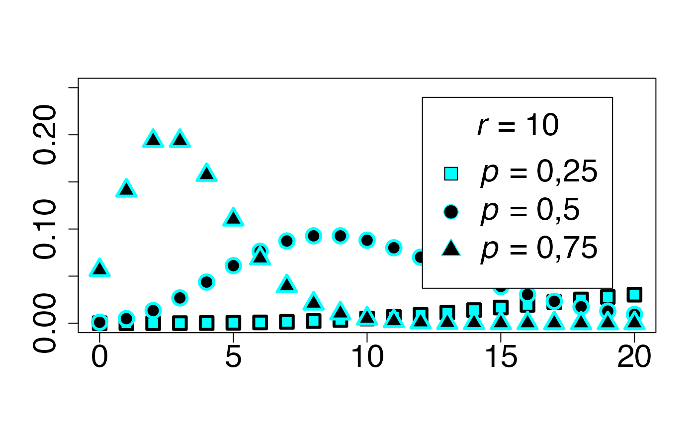
#>       2

Loi négative binomiale (cas asymétrique)

Chemin = "~/Documents/Recherche/DeBoeck/Graphes/Fichiers/"
colmodel="cmyk"
pdf(file = paste(Chemin,"dens_",LOI,".pdf",sep=""),
    width = 8, height = 7, onefile = TRUE, family = "Helvetica",
    title = "Probability or cumulative distribution graphs", paper = "special", colormodel = colmodel)
infx=0;supx=20;
infy=0;supy=0.25;
fd <- function(x) {dnbinom(x,10,0.25)}
plot(cbind(0:20,sapply(0:20,fd)),xlim=c(infx,supx),ylim=c(infy,supy),type="p",ylab="",xlab="",pch=22,bg=bgmagentas[1],cex=2,lwd=3,col=colmagentas[1],cex.axis=2)
fd <- function(x) {dnbinom(x,10,0.5)}
points(cbind(0:20,sapply(0:20,fd)),xlim=c(infx,supx),ylim=c(infy,supy),type="p",ylab="",xlab="",pch=21,bg=bgmagentas[2],cex=2,lwd=3,col=colmagentas[2],new=T)
fd <- function(x) {dnbinom(x,10,0.75)}
points(cbind(0:20,sapply(0:20,fd)),xlim=c(infx,supx),ylim=c(infy,supy),type="p",ylab="",xlab="",pch=24,bg=bgmagentas[3],cex=2,lwd=3,col=colmagentas[3],new=T)
leg.txt <- c(expression(paste(italic(p)," = 0,25",sep="")), expression(paste(italic(p)," = 0,5",sep="")),
             expression(paste(italic(p)," = 0,75",sep="")))
legend("topright", leg.txt, title = expression(paste(italic(r)," = 10",sep="")) , pch = c(22, 21, 24), col = c(colmagentas[1],colmagentas[2],colmagentas[3]), pt.bg = c(bgmagentas[1],bgmagentas[2],bgmagentas[3]), cex = 2, bg="white", inset=.075)# , pch = "*"
dev.off()
#> agg_png 
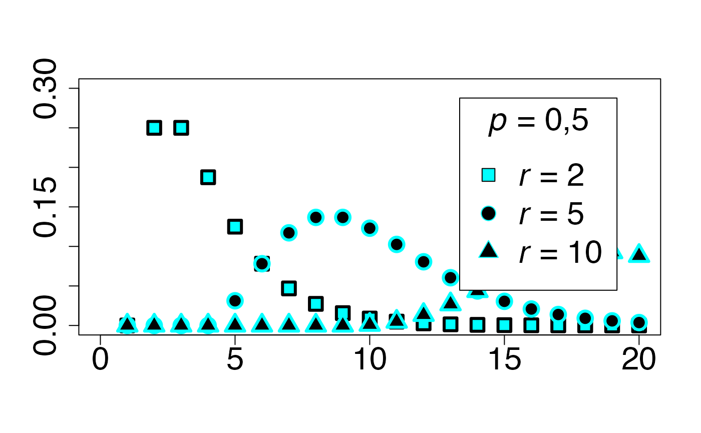
#>       2

Loi de Pascal (cas symétrique)

Chemin = "~/Documents/Recherche/DeBoeck/Graphes/Fichiers/"
colmodel="cmyk"
pdf(file = paste(Chemin,"dens_",LOI,".pdf",sep=""),
    width = 8, height = 7, onefile = TRUE, family = "Helvetica",
    title = "Probability or cumulative distribution graphs", paper = "special", colormodel = colmodel)
infx=0;supx=20;
infy=0;supy=0.3;
dpascal <- function(x,p,r) (choose(x-1,r-1)*(1-p)^(x-r)*p^(r))
fd <- function(x) {dpascal(x,0.5,2)}
plot(cbind(0:20,sapply(0:20,fd)),xlim=c(infx,supx),ylim=c(infy,supy),type="p",ylab="",xlab="",pch=22,bg=bgmagentas[1],cex=2,lwd=3,col=colmagentas[1],cex.axis=2)
fd <- function(x) {dpascal(x,0.5,5)}
points(cbind(0:20,sapply(0:20,fd)),xlim=c(infx,supx),ylim=c(infy,supy),type="p",ylab="",xlab="",pch=21,bg=bgmagentas[2],cex=2,lwd=3,col=colmagentas[2],new=T)
fd <- function(x) {dpascal(x,0.5,10)}
points(cbind(0:20,sapply(0:20,fd)),xlim=c(infx,supx),ylim=c(infy,supy),type="p",ylab="",xlab="",pch=24,bg=bgmagentas[3],cex=2,lwd=3,col=colmagentas[3],new=T)
leg.txt <- c(expression(paste(italic(r)," = 2",sep="")), expression(paste(italic(r)," = 5",sep="")),
             expression(paste(italic(r)," = 10",sep="")))
legend("topright", leg.txt, title = expression(paste(italic(p)," = 0,5",sep="")) , pch = c(22, 21, 24), col = c(colmagentas[1],colmagentas[2],colmagentas[3]), pt.bg = c(bgmagentas[1],bgmagentas[2],bgmagentas[3]), cex = 2, bg="white", inset=.075)# , pch = "*"
dev.off()
#> agg_png 
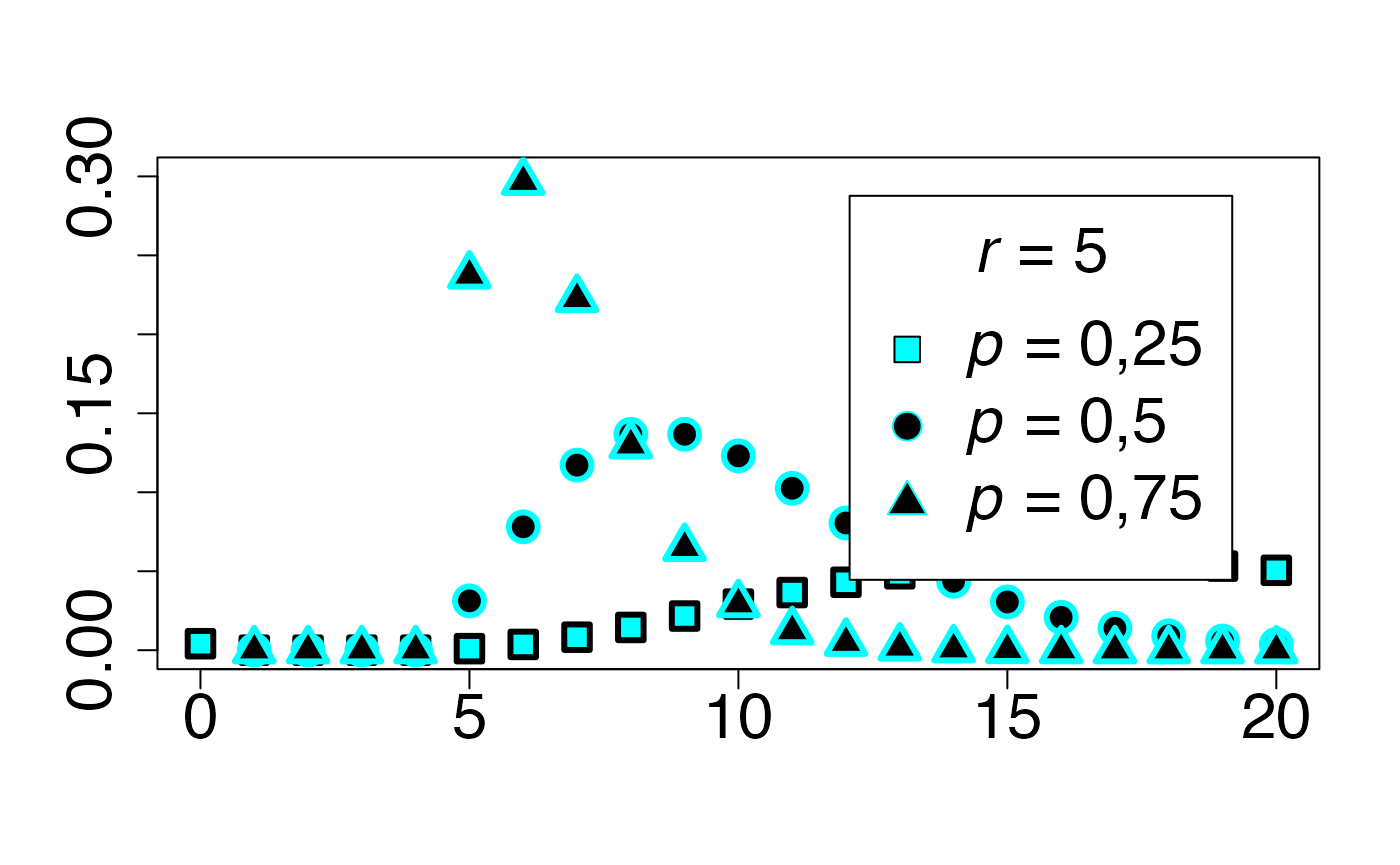
#>       2

Loi de Pascal (cas asymétrique)

Chemin = "~/Documents/Recherche/DeBoeck/Graphes/Fichiers/"
colmodel="cmyk"
pdf(file = paste(Chemin,"dens_",LOI,".pdf",sep=""),
    width = 8, height = 7, onefile = TRUE, family = "Helvetica",
    title = "Probability or cumulative distribution graphs", paper = "special", colormodel = colmodel)
infx=0;supx=20;
infy=0;supy=0.3;
dpascal <- function(x,p,r) (choose(x-1,r-1)*(1-p)^(x-r)*p^(r))
fd <- function(x) {dpascal(x,0.25,5)}
plot(cbind(0:20,sapply(0:20,fd)),xlim=c(infx,supx),ylim=c(infy,supy),type="p",ylab="",xlab="",pch=22,bg=bgmagentas[1],cex=2,lwd=3,col=colmagentas[1],cex.axis=2)
fd <- function(x) {dpascal(x,0.5,5)}
points(cbind(0:20,sapply(0:20,fd)),xlim=c(infx,supx),ylim=c(infy,supy),type="p",ylab="",xlab="",pch=21,bg=bgmagentas[2],cex=2,lwd=3,col=colmagentas[2],new=T)
fd <- function(x) {dpascal(x,0.75,5)}
points(cbind(0:20,sapply(0:20,fd)),xlim=c(infx,supx),ylim=c(infy,supy),type="p",ylab="",xlab="",pch=24,bg=bgmagentas[3],cex=2,lwd=3,col=colmagentas[3],new=T)
leg.txt <- c(expression(paste(italic(p)," = 0,25",sep="")), expression(paste(italic(p)," = 0,5",sep="")),
             expression(paste(italic(p)," = 0,75",sep="")))
legend("topright", leg.txt, title = expression(paste(italic(r)," = 5",sep="")) , pch = c(22, 21, 24), col = c(colmagentas[1],colmagentas[2],colmagentas[3]), pt.bg = c(bgmagentas[1],bgmagentas[2],bgmagentas[3]), cex = 2, bg="white", inset=.075)# , pch = "*"
dev.off()
#> agg_png 
#>       2

Loi hypergéométrique (en fonction de $N$)

Chemin = "~/Documents/Recherche/DeBoeck/Graphes/Fichiers/"
colmodel="cmyk"
pdf(file = paste(Chemin,"dens_",LOI,".pdf",sep=""),
    width = 8, height = 7, onefile = TRUE, family = "Helvetica",
    title = "Probability or cumulative distribution graphs", paper = "special", colormodel = colmodel)
infx=0;supx=10;
infy=0;supy=0.5;
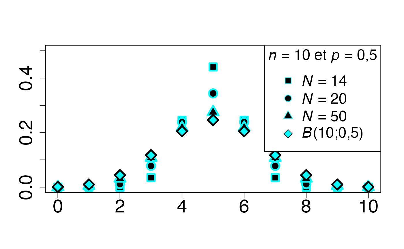
dhypergeom <- function(x,N,n,p) (choose(N*p,x)*choose(N*(1-p),n-x)/choose(N,n))
fd <- function(x) {dhypergeom(x,14,10,0.5)}
plot(cbind(0:10,sapply(0:10,fd)),xlim=c(infx,supx),ylim=c(infy,supy),type="p",ylab="",xlab="",pch=22,bg=bgmagentas[1],cex=2,lwd=3,col=colmagentas[4],cex.axis=2)
fd <- function(x) {dhypergeom(x,20,10,0.5)}
points(cbind(0:10,sapply(0:10,fd)),xlim=c(infx,supx),ylim=c(infy,supy),type="p",ylab="",xlab="",pch=21,bg=bgmagentas[2],cex=2,lwd=3,col=colmagentas[3],new=T)
fd <- function(x) {dhypergeom(x,50,10,0.5)}
points(cbind(0:10,sapply(0:10,fd)),xlim=c(infx,supx),ylim=c(infy,supy),type="p",ylab="",xlab="",pch=24,bg=bgmagentas[3],cex=2,lwd=3,col=colmagentas[2],new=T)
fd <- function(x) {dbinom(x,10,0.5)}
points(cbind(0:10,sapply(0:10,fd)),xlim=c(infx,supx),ylim=c(infy,supy),type="p",ylab="",xlab="",pch=23,bg=bgmagentas[1],cex=2,lwd=3,col=colmagentas[1],new=T)
leg.txt <- c(expression(paste(italic(N)," = 14",sep="")), expression(paste(italic(N)," = 20",sep="")),
             expression(paste(italic(N)," = 50",sep="")), expression(paste(italic(B),"(10;0,5)",sep="")))
legend("topright", leg.txt, title = expression(paste(italic(n), " = 10 et ", italic(p)," = 0,5",sep="")), pch = c(22, 21, 24, 23), col = c(colmagentas[4],colmagentas[3],colmagentas[2],colmagentas[1]), pt.bg = c(bgmagentas[4],bgmagentas[3],bgmagentas[2],bgmagentas[1]), cex = 1.6, bg="white", inset=.0)# , pch = "*"
dev.off()
#> agg_png 
#>       2

Loi hypergéométrique (en fonction de $n$)

Chemin = "~/Documents/Recherche/DeBoeck/Graphes/Fichiers/"
colmodel="cmyk"
pdf(file = paste(Chemin,"dens_",LOI,".pdf",sep=""),
    width = 8, height = 7, onefile = TRUE, family = "Helvetica",
    title = "Probability or cumulative distribution graphs", paper = "special", colormodel = colmodel)
infx=0;supx=15;
infy=0;supy=0.4;
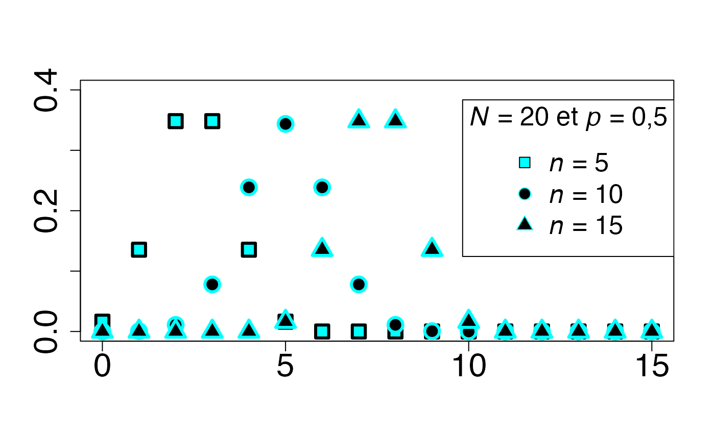
dhypergeom <- function(x,N,n,p) (choose(N*p,x)*choose(N*(1-p),n-x)/choose(N,n))
fd <- function(x) {dhypergeom(x,20,5,0.5)}
plot(cbind(0:15,sapply(0:15,fd)),xlim=c(infx,supx),ylim=c(infy,supy),type="p",ylab="",xlab="",pch=22,bg=bgmagentas[1],cex=2,lwd=3,col=colmagentas[1],cex.axis=2)
fd <- function(x) {dhypergeom(x,20,10,0.5)}
points(cbind(0:15,sapply(0:15,fd)),xlim=c(infx,supx),ylim=c(infy,supy),type="p",ylab="",xlab="",pch=21,bg=bgmagentas[2],cex=2,lwd=3,col=colmagentas[2],new=T)
fd <- function(x) {dhypergeom(x,20,15,0.5)}
points(cbind(0:15,sapply(0:15,fd)),xlim=c(infx,supx),ylim=c(infy,supy),type="p",ylab="",xlab="",pch=24,bg=bgmagentas[3],cex=2,lwd=3,col=colmagentas[3],new=T)
leg.txt <- c(expression(paste(italic(n)," = 5",sep="")), expression(paste(italic(n)," = 10",sep="")),
             expression(paste(italic(n)," = 15",sep="")))
legend("topright", leg.txt, title = expression(paste(italic(N), " = 20 et ", italic(p)," = 0,5",sep="")) , pch = c(22, 21, 24, 23), col = c(colmagentas[1],colmagentas[2],colmagentas[3],colmagentas[4]), pt.bg = c(bgmagentas[1],bgmagentas[2],bgmagentas[3],bgmagentas[4]), cex = 1.6, bg="white", inset=c(0,.075))# , pch = "*"
dev.off()
#> agg_png 
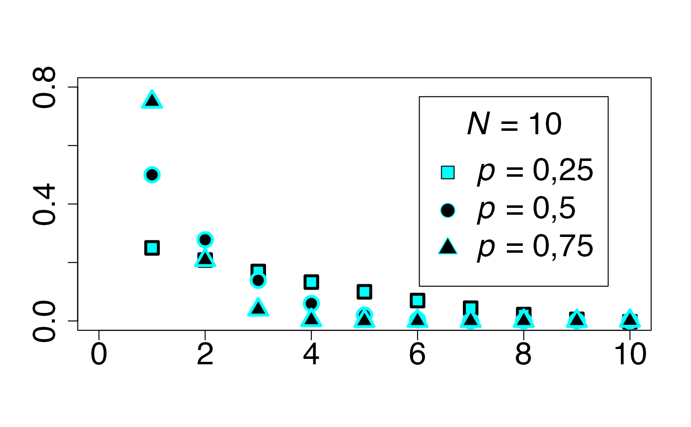
#>       2

Loi hypergéométrique (en fonction de $p$)

Chemin = "~/Documents/Recherche/DeBoeck/Graphes/Fichiers/"
colmodel="cmyk"
pdf(file = paste(Chemin,"dens_",LOI,".pdf",sep=""),
    width = 8, height = 7, onefile = TRUE, family = "Helvetica",
    title = "Probability or cumulative distribution graphs", paper = "special", colormodel = colmodel)
infx=0;supx=10;
infy=0;supy=0.52;
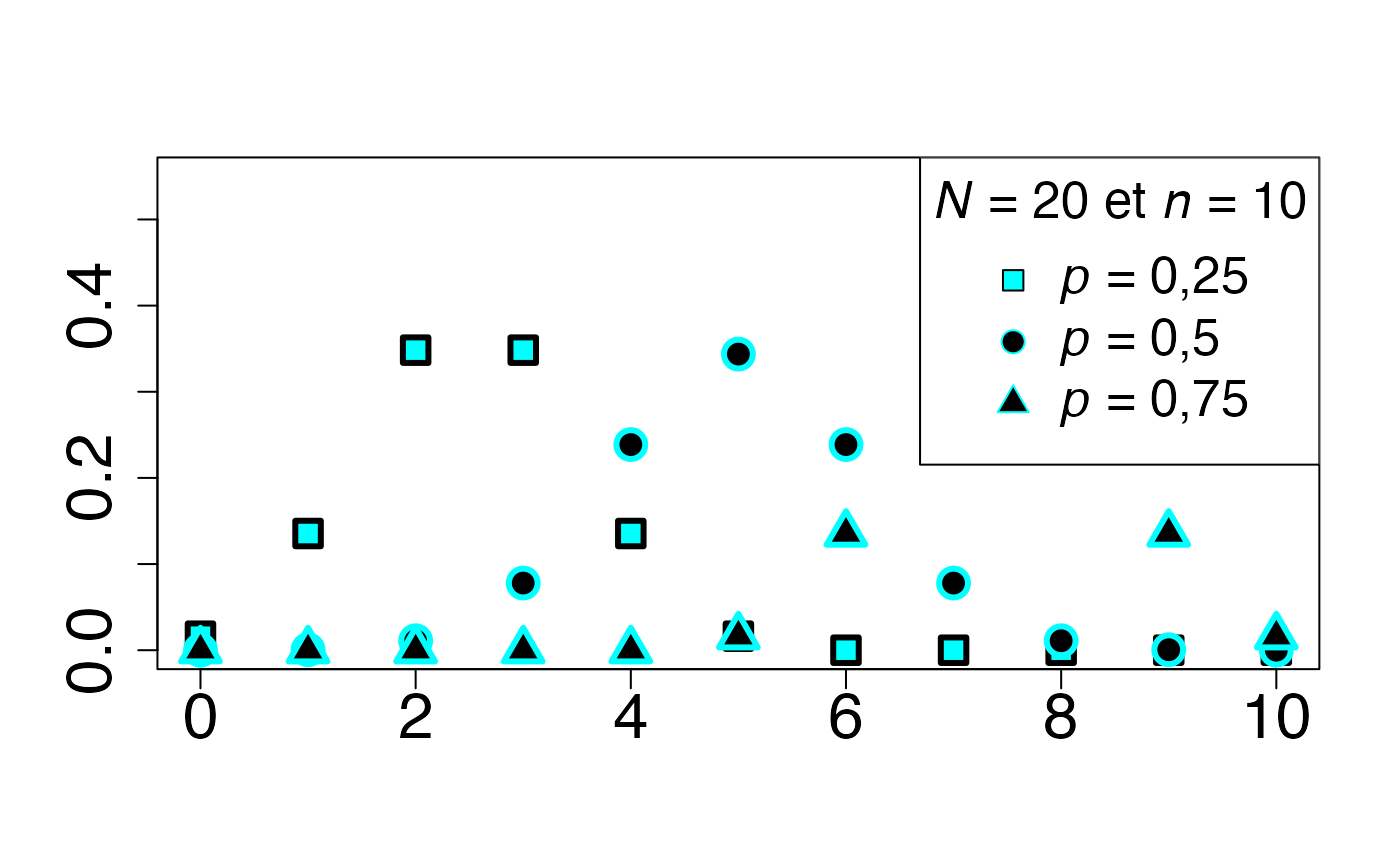
dhypergeom <- function(x,N,n,p) (choose(N*p,x)*choose(N*(1-p),n-x)/choose(N,n))
fd <- function(x) {dhypergeom(x,20,10,0.25)}
plot(cbind(0:10,sapply(0:10,fd)),xlim=c(infx,supx),ylim=c(infy,supy),type="p",ylab="",xlab="",pch=22,bg=bgmagentas[1],cex=2,lwd=3,col=colmagentas[1],cex.axis=2)
fd <- function(x) {dhypergeom(x,20,10,0.5)}
points(cbind(0:10,sapply(0:10,fd)),xlim=c(infx,supx),ylim=c(infy,supy),type="p",ylab="",xlab="",pch=21,bg=bgmagentas[2],cex=2,lwd=3,col=colmagentas[2],new=T)
fd <- function(x) {dhypergeom(x,20,10,0.75)}
points(cbind(0:10,sapply(0:10,fd)),xlim=c(infx,supx),ylim=c(infy,supy),type="p",ylab="",xlab="",pch=24,bg=bgmagentas[3],cex=2,lwd=3,col=colmagentas[3],new=T)
leg.txt <- c(expression(paste(italic(p)," = 0,25",sep="")), expression(paste(italic(p)," = 0,5",sep="")),
             expression(paste(italic(p)," = 0,75",sep="")))
legend("topright", leg.txt, title = expression(paste(italic(N), " = 20 et ", italic(n)," = 10",sep="")) , pch = c(22, 21, 24, 23), pt.bg = c(bgmagentas[1],bgmagentas[2],bgmagentas[3],bgmagentas[4]), col = c(colmagentas[1],colmagentas[2],colmagentas[3],colmagentas[4]), cex = 1.6, bg="white", inset=c(0,0))# , pch = "*"
dev.off()
#> agg_png 
#>       2

Loi d’un temps d’arrêt (en fonction de $N$)

Chemin = "~/Documents/Recherche/DeBoeck/Graphes/Fichiers/"
colmodel="cmyk"
pdf(file = paste(Chemin,"dens_",LOI,".pdf",sep=""),
    width = 8, height = 7, onefile = TRUE, family = "Helvetica",
    title = "Probability or cumulative distribution graphs", paper = "special", colormodel = colmodel)
infx=0;supx=10;
infy=0;supy=0.6;
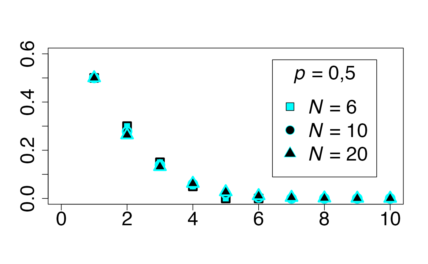
darret <- function(x,N,p) (choose(N*(1-p),x-1)/choose(N,x)*N*p/x)
fd <- function(x) {darret(x,6,0.5)}
plot(cbind(0:10,sapply(0:10,fd)),xlim=c(infx,supx),ylim=c(infy,supy),type="p",ylab="",xlab="",pch=22,bg=bgmagentas[1],cex=2,lwd=3,col=colmagentas[1],cex.axis=2)
fd <- function(x) {darret(x,10,0.5)}
points(cbind(0:10,sapply(0:10,fd)),xlim=c(infx,supx),ylim=c(infy,supy),type="p",ylab="",xlab="",pch=21,bg=bgmagentas[2],cex=2,lwd=3,col=colmagentas[2],new=T)
fd <- function(x) {darret(x,20,0.5)}
points(cbind(0:10,sapply(0:10,fd)),xlim=c(infx,supx),ylim=c(infy,supy),type="p",ylab="",xlab="",pch=24,bg=bgmagentas[3],cex=2,lwd=3,col=colmagentas[3],new=T)
leg.txt <- c(expression(paste(italic(N)," = 6",sep="")), expression(paste(italic(N)," = 10",sep="")),
             expression(paste(italic(N)," = 20",sep="")))
legend("topright", leg.txt, title = expression(paste(italic(p)," = 0,5",sep="")) , pch = c(22, 21, 24), col = c(colmagentas[1],colmagentas[2],colmagentas[3]), pt.bg = c(bgmagentas[1],bgmagentas[2],bgmagentas[3]), cex = 2, bg="white", inset=.075)# , pch = "*"
dev.off()
#> agg_png 
#>       2

Loi d’un temps d’arrêt (en fonction de $p$)

Chemin = "~/Documents/Recherche/DeBoeck/Graphes/Fichiers/"
colmodel="cmyk"
pdf(file = paste(Chemin,"dens_",LOI,".pdf",sep=""),
    width = 8, height = 7, onefile = TRUE, family = "Helvetica",
    title = "Probability or cumulative distribution graphs", paper = "special", colormodel = colmodel)
infx=0;supx=10;
infy=0;supy=0.8;
darret <- function(x,N,p) (choose(N*(1-p),x-1)/choose(N,x)*N*p/x)
fd <- function(x) {darret(x,10,0.25)}
plot(cbind(0:10,sapply(0:10,fd)),xlim=c(infx,supx),ylim=c(infy,supy),type="p",ylab="",xlab="",pch=22,bg=bgmagentas[1],cex=2,lwd=3,col=colmagentas[1],cex.axis=2)
fd <- function(x) {darret(x,10,0.5)}
points(cbind(0:10,sapply(0:10,fd)),xlim=c(infx,supx),ylim=c(infy,supy),type="p",ylab="",xlab="",pch=21,bg=bgmagentas[2],cex=2,lwd=3,col=colmagentas[2],new=T)
fd <- function(x) {darret(x,10,0.75)}
points(cbind(0:10,sapply(0:10,fd)),xlim=c(infx,supx),ylim=c(infy,supy),type="p",ylab="",xlab="",pch=24,bg=bgmagentas[3],cex=2,lwd=3,col=colmagentas[3],new=T)
leg.txt <- c(expression(paste(italic(p)," = 0,25",sep="")), expression(paste(italic(p)," = 0,5",sep="")),
             expression(paste(italic(p)," = 0,75",sep="")))
legend("topright", leg.txt, title = expression(paste(italic(N)," = 10",sep="")) , pch = c(22, 21, 24), col = c(colmagentas[1],colmagentas[2],colmagentas[3]), pt.bg = c(bgmagentas[1],bgmagentas[2],bgmagentas[3]), cex = 2, bg="white", inset=.075)# , pch = "*"
dev.off()
#> agg_png 
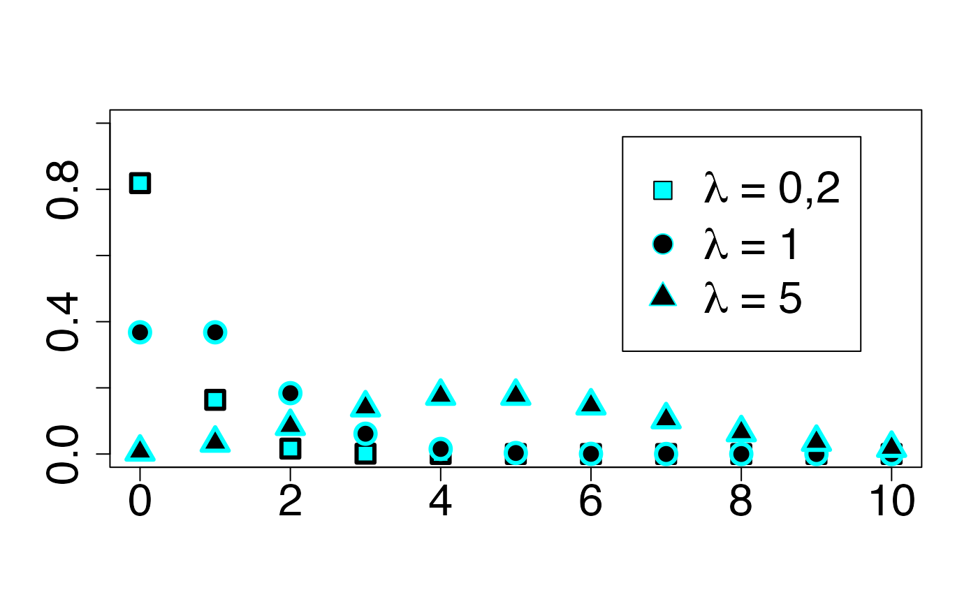
#>       2

Loi de Poisson

Chemin = "~/Documents/Recherche/DeBoeck/Graphes/Fichiers/"
colmodel="cmyk"
pdf(file = paste(Chemin,"dens_",LOI,".pdf",sep=""),
    width = 8, height = 7, onefile = TRUE, family = "Helvetica",
    title = "Probability or cumulative distribution graphs", paper = "special", colormodel = colmodel)
infx=0;supx=10;
infy=0;supy=1;
fd <- function(x) {dpois(x,0.2)}
plot(cbind(0:20,sapply(0:20,fd)),xlim=c(infx,supx),ylim=c(infy,supy),type="p",ylab="",xlab="",pch=22,bg=bgmagentas[1],cex=2,lwd=3,col=colmagentas[1],cex.axis=2)
fd <- function(x) {dpois(x,1)}
points(cbind(0:20,sapply(0:20,fd)),xlim=c(infx,supx),ylim=c(infy,supy),type="p",ylab="",xlab="",pch=21,bg=bgmagentas[2],cex=2,lwd=3,col=colmagentas[2],new=T)
fd <- function(x) {dpois(x,5)}
points(cbind(0:20,sapply(0:20,fd)),xlim=c(infx,supx),ylim=c(infy,supy),type="p",ylab="",xlab="",pch=24,bg=bgmagentas[3],cex=2,lwd=3,col=colmagentas[3],new=T)
leg.txt <- c(expression(paste(lambda," = 0,2",sep="")), expression(paste(lambda," = 1",sep="")),
             expression(paste(lambda," = 5",sep="")))
legend("topright", leg.txt, pch = c(22, 21, 24), col = c(colmagentas[1],colmagentas[2],colmagentas[3]), pt.bg = c(bgmagentas[1],bgmagentas[2],bgmagentas[3]), cex = 2, bg="white", inset=.075)# , pch = "*"
dev.off()
#> agg_png 
#>       2

Représentations graphiques de lois continues

Loi uniforme continue

Fonction de densité de probabilité

Chemin = "~/Documents/Recherche/DeBoeck/Graphes/Fichiers/"
colmodel="cmyk"
pdf(file = paste(Chemin,"dens_",LOI,".pdf",sep=""),
    width = 8, height = 7, onefile = TRUE, family = "Helvetica",
    title = "Probability or cumulative distribution graphs", paper = "special", colormodel = colmodel)
curve(fdunif,from=-3,to=3,type="n",ylab="",xlab="",lty=1,lwd=3,cex.axis=2)
curve(fdunif,from=-2,to=2,add=TRUE,lty=1,lwd=3)
curve(fdunif,from=-3,to=-2.000000001,add=TRUE,lty=1,lwd=3)
curve(fdunif,from=2.00000001,to=3,add=TRUE,lty=1,lwd=3)
dev.off()
#> agg_png 
#>       2

Fonction de répartition

Chemin = "~/Documents/Recherche/DeBoeck/Graphes/Fichiers/"
colmodel="cmyk"
pdf(file = paste(Chemin,"frep_",LOI,".pdf",sep=""),
    width = 8, height = 7, onefile = TRUE, family = "Helvetica",
    title = "Probability or cumulative distribution graphs", paper = "special", colormodel = colmodel)
curve(frunif,from=-3,to=3,ylab="",xlab="",lty=1,lwd=3,cex.axis=2)
dev.off()
#> agg_png 
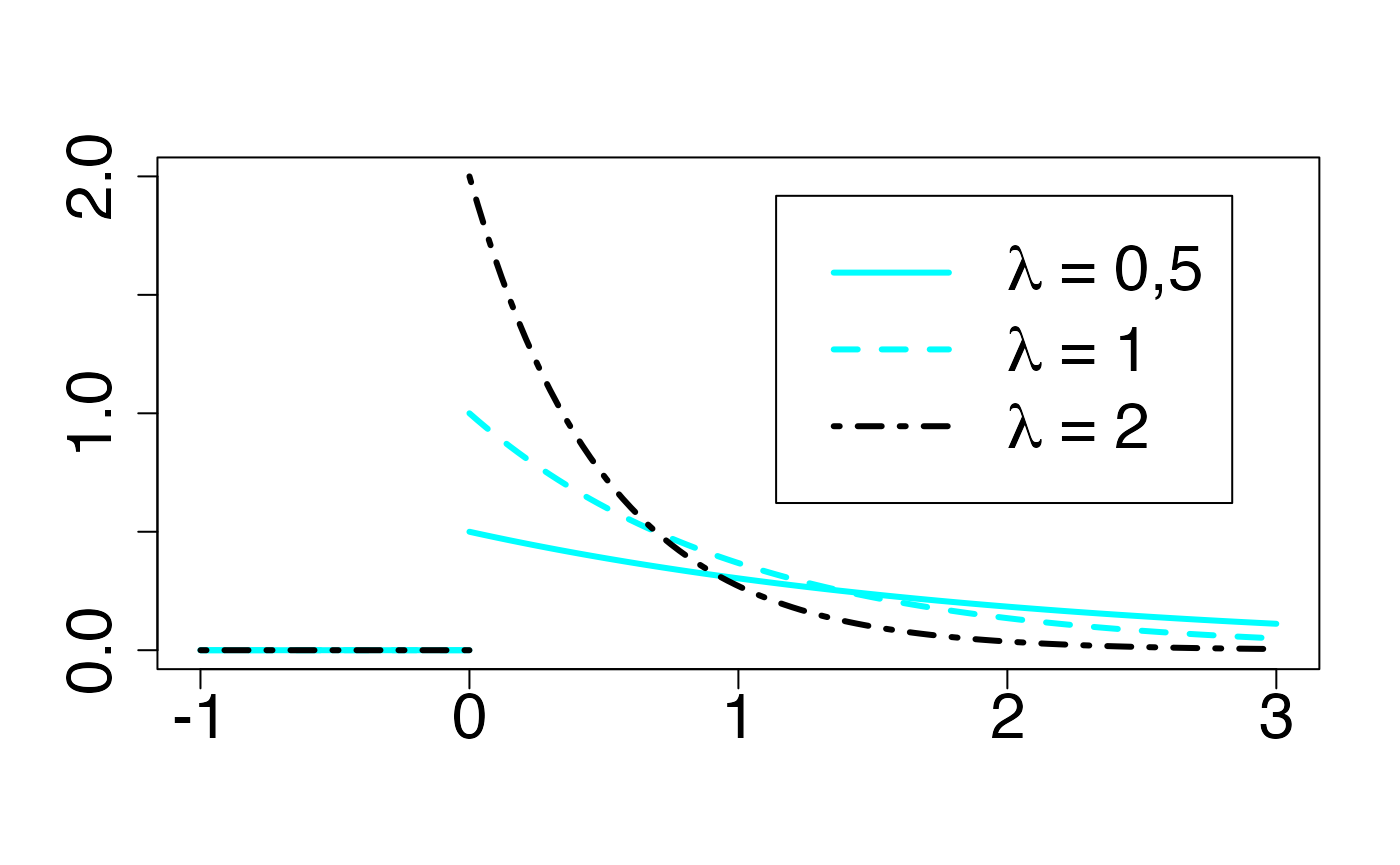
#>       2

Loi exponentielle

Fonction de densité de probabilité

Chemin = "~/Documents/Recherche/DeBoeck/Graphes/Fichiers/"
colmodel="cmyk"
pdf(file = paste(Chemin,"dens_",LOI,".pdf",sep=""),
    width = 8, height = 7, onefile = TRUE, family = "Helvetica",
    title = "Probability or cumulative distribution graphs", paper = "special", colormodel = colmodel)
infx=-1;supx=3;
fd <- function(x) {dexp(x,2)}
curve(fd,from=infx,to=supx,type="n",ylab="",xlab="",lty=4,lwd=3,col=colmagentas[1],cex.axis=2)
fd <- function(x) {dexp(x,0.5)}
curve(fd,from=infx,to=-0.00001,ylab="",xlab="",lty=1,lwd=3,col=colmagentas[3],add=TRUE)
curve(fd,from=0.00001,to=supx,ylab="",xlab="",lty=1,lwd=3,col=colmagentas[3],add=TRUE)
fd <- function(x) {dexp(x,1)}
curve(fd,from=infx,to=-0.00001,ylab="",xlab="",lty=2,lwd=3,col=colmagentas[2],add=TRUE)
curve(fd,from=0.00001,to=supx,ylab="",xlab="",lty=2,lwd=3,col=colmagentas[2],add=TRUE)
fd <- function(x) {dexp(x,2)}
curve(fd,from=infx,to=-0.00001,ylab="",xlab="",lty=4,lwd=3,col=colmagentas[1],add=TRUE)
curve(fd,from=0.00001,to=supx,ylab="",xlab="",lty=4,lwd=3,col=colmagentas[1],add=TRUE)
leg.txt <- c(expression(paste(lambda," = 0,5",sep="")), expression(paste(lambda," = 1",sep="")),
             expression(paste(lambda," = 2",sep="")))
legend("topright", leg.txt, lty = c(1, 2, 4), lwd=3, col = c(colmagentas[3],colmagentas[2],colmagentas[1]), cex = 2, bg="white", inset=.075)# , pch = "*"
dev.off()
#> agg_png 
#>       2

Fonction de répartition

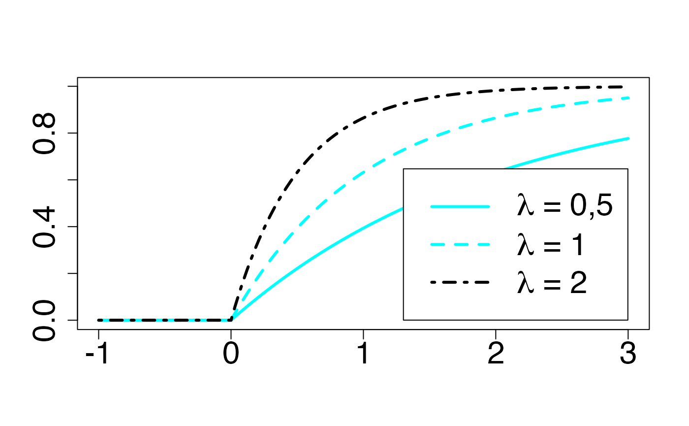
Chemin = "~/Documents/Recherche/DeBoeck/Graphes/Fichiers/"
colmodel="cmyk"
pdf(file = paste(Chemin,"frep_",LOI,".pdf",sep=""),
    width = 8, height = 7, onefile = TRUE, family = "Helvetica",
    title = "Probability or cumulative distribution graphs", paper = "special",colormodel = colmodel)
infx=-1;supx=3;
fr <- function(x) {pexp(x,2)}
curve(fr,from=infx,to=supx,ylab="",xlab="",lty=4,lwd=3,col=colmagentas[1],type="n",cex.axis=2)
fr <- function(x) {pexp(x,0.5)}
curve(fr,from=infx,to=0,ylab="",xlab="",lty=1,lwd=3,add=T,col=colmagentas[3])
curve(fr,from=0,to=supx,ylab="",xlab="",lty=1,lwd=3,add=T,col=colmagentas[3])
fr <- function(x) {pexp(x,1)}
curve(fr,from=infx,to=0,ylab="",xlab="",lty=2,lwd=3,add=T,col=colmagentas[2])
curve(fr,from=0,to=supx,ylab="",xlab="",lty=2,lwd=3,add=T,col=colmagentas[2])
fr <- function(x) {pexp(x,2)}
curve(fr,from=infx,to=0,ylab="",xlab="",lty=4,lwd=3,col=colmagentas[1],add=T)
curve(fr,from=0,to=supx,ylab="",xlab="",lty=4,lwd=3,col=colmagentas[1],add=T)
leg.txt <- c(expression(paste(lambda," = 0,5",sep="")), expression(paste(lambda," = 1",sep="")),
             expression(paste(lambda," = 2",sep="")))
legend("bottomright", leg.txt, lty = c(1, 2, 4), lwd=3, col = c(colmagentas[3],colmagentas[2],colmagentas[1]), cex = 2, bg="white", inset=.0375)# , pch = "*"
dev.off()
#> agg_png 
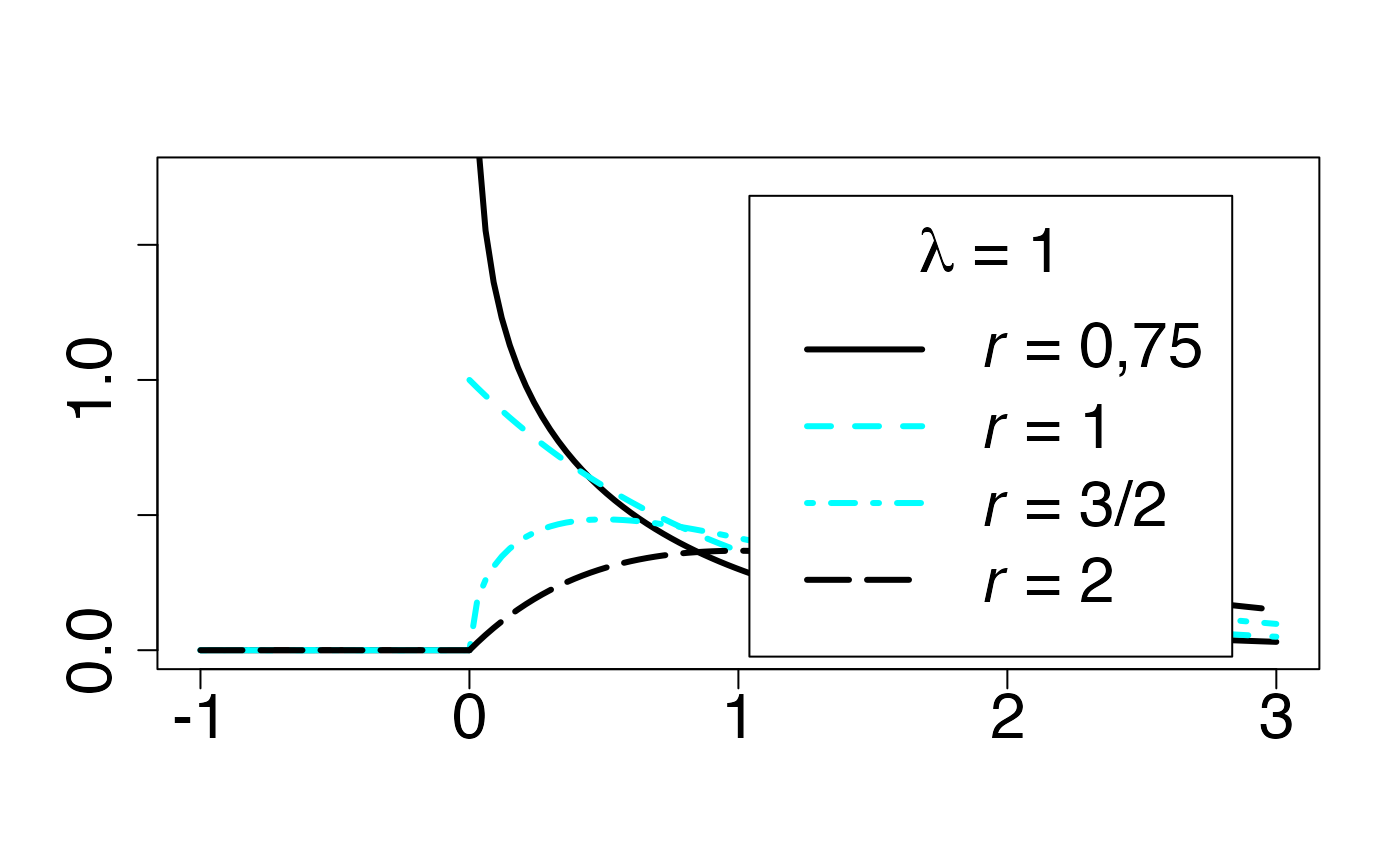
#>       2

Loi gamma (en fonction de $r$)

Fonction de densité de probabilité

Chemin = "~/Documents/Recherche/DeBoeck/Graphes/Fichiers/"
colmodel="cmyk"
pdf(file = paste(Chemin,"dens_",LOI,".pdf",sep=""),
    width = 8, height = 7, onefile = TRUE, family = "Helvetica",
    title = "Probability or cumulative distribution graphs", paper = "special", colormodel = colmodel)
infx=-1;supx=3;
fd <- function(x) {dgamma(x,0.75)}
curve(fd,from=infx,to=supx,ylab="",xlab="",lty=1,lwd=3,col=colmagentas[1],type="n",cex.axis=2)
curve(fd,from=infx,to=-0.000001,ylab="",xlab="",lty=1,lwd=3,col=colmagentas[1],add=T)
curve(fd,from=0.000001,to=supx,ylab="",xlab="",lty=1,lwd=3,col=colmagentas[1],add=T)
fd <- function(x) {dgamma(x,1)}
curve(fd,from=infx,to=-0.000001,ylab="",xlab="",lty=2,lwd=3,add=T,col=colmagentas[2])
curve(fd,from=0.000001,to=supx,ylab="",xlab="",lty=2,lwd=3,add=T,col=colmagentas[2])
fd <- function(x) {dgamma(x,1.5)}
curve(fd,from=infx,to=-0.000001,ylab="",xlab="",lty=4,lwd=3,add=T,col=colmagentas[3])
curve(fd,from=0.000001,to=supx,ylab="",xlab="",lty=4,lwd=3,add=T,col=colmagentas[3])
fd <- function(x) {dgamma(x,2)}
curve(fd,from=infx,to=-0.000001,ylab="",xlab="",lty=5,lwd=3,add=T,col=colmagentas[1])
curve(fd,from=0.000001,to=supx,ylab="",xlab="",lty=5,lwd=3,add=T,col=colmagentas[1])
leg.txt <- c(expression(paste(italic(r)," = 0,75")), expression(paste(italic(r)," = 1")), expression(paste(italic(r)," = 3/2")),
             expression(paste(italic(r)," = 2")))
legend("topright", leg.txt, title = expression(paste(lambda," = 1",sep="")), lty = c(1, 2, 4,5), lwd=3, col = c(colmagentas[1],colmagentas[2],colmagentas[3],colmagentas[1]), cex = 2, bg="white", inset=.075)# , pch = "*"
dev.off()
#> agg_png 
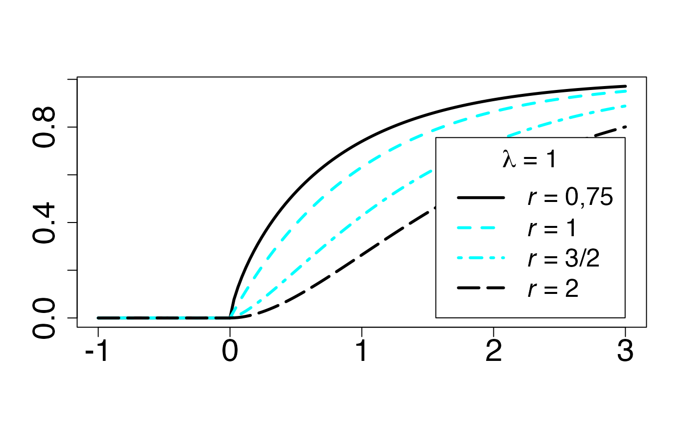
#>       2

Fonction de répartition

Chemin = "~/Documents/Recherche/DeBoeck/Graphes/Fichiers/"
colmodel="cmyk"
pdf(file = paste(Chemin,"frep_",LOI,".pdf",sep=""),
    width = 8, height = 7, onefile = TRUE, family = "Helvetica",
    title = "Probability or cumulative distribution graphs", paper = "special", colormodel = colmodel)
infx=-1;supx=3;
fr <- function(x) {pgamma(x,0.75)}
curve(fr,from=infx,to=supx,ylab="",xlab="",lty=1,lwd=3,col=colmagentas[1],type="n",cex.axis=2)
curve(fr,from=infx,to=0,ylab="",xlab="",lty=1,lwd=3,col=colmagentas[1],add=T)
curve(fr,from=0,to=supx,ylab="",xlab="",lty=1,lwd=3,col=colmagentas[1],add=T)
fr <- function(x) {pgamma(x,1)}
curve(fr,from=infx,to=0,ylab="",xlab="",lty=2,lwd=3,add=T,col=colmagentas[2])
curve(fr,from=0,to=supx,ylab="",xlab="",lty=2,lwd=3,add=T,col=colmagentas[2])
fr <- function(x) {pgamma(x,1.5)}
curve(fr,from=infx,to=0,ylab="",xlab="",lty=4,lwd=3,add=T,col=colmagentas[3])
curve(fr,from=0,to=supx,ylab="",xlab="",lty=4,lwd=3,add=T,col=colmagentas[3])
fr <- function(x) {pgamma(x,2)}
curve(fr,from=infx,to=0,ylab="",xlab="",lty=5,lwd=3,add=T,col=colmagentas[1])
curve(fr,from=0,to=supx,ylab="",xlab="",lty=5,lwd=3,add=T,col=colmagentas[1])
leg.txt <- c(expression(paste(italic(r)," = 0,75")), expression(paste(italic(r)," = 1")), expression(paste(italic(r)," = 3/2")),
             expression(paste(italic(r)," = 2")))
legend("bottomright", leg.txt, title = expression(paste(lambda," = 1",sep="")), lty = c(1, 2, 4,5), lwd=3, col = c(colmagentas[1],colmagentas[2],colmagentas[3],colmagentas[1]), cex = 1.6, bg="white", inset=.0375)# , pch = "*"
dev.off()
#> agg_png 
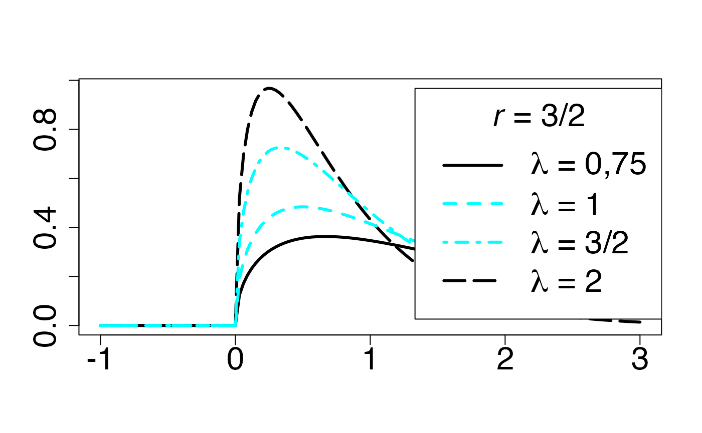
#>       2

Loi gamma (en fonction de $lambda$)

Fonction de densité de probabilité

Chemin = "~/Documents/Recherche/DeBoeck/Graphes/Fichiers/"
colmodel="cmyk"
pdf(file = paste(Chemin,"dens_",LOI,".pdf",sep=""),
    width = 8, height = 7, onefile = TRUE, family = "Helvetica",
    title = "Probability or cumulative distribution graphs", paper = "special", colormodel = colmodel)
infx=-1;supx=3;
fd <- function(x) {dgamma(x,1.5,2)}
curve(fd,from=infx,to=supx,ylab="",xlab="",lty=1,lwd=3,col=colmagentas[1],type="n",cex.axis=2)
curve(fd,from=infx,to=-0.000001,ylab="",xlab="",lty=5,lwd=3,add=T,col=colmagentas[1])
curve(fd,from=0.000001,to=supx,ylab="",xlab="",lty=5,lwd=3,add=T,col=colmagentas[1])
fd <- function(x) {dgamma(x,1.5,0.75)}
curve(fd,from=infx,to=-0.000001,ylab="",xlab="",lty=1,lwd=3,col=colmagentas[1],add=T)
curve(fd,from=0.000001,to=supx,ylab="",xlab="",lty=1,lwd=3,col=colmagentas[1],add=T)
fd <- function(x) {dgamma(x,1.5,1)}
curve(fd,from=infx,to=-0.000001,ylab="",xlab="",lty=2,lwd=3,add=T,col=colmagentas[2])
curve(fd,from=0.000001,to=supx,ylab="",xlab="",lty=2,lwd=3,add=T,col=colmagentas[2])
fd <- function(x) {dgamma(x,1.5,1.5)}
curve(fd,from=infx,to=-0.000001,ylab="",xlab="",lty=4,lwd=3,add=T,col=colmagentas[3])
curve(fd,from=0.000001,to=supx,ylab="",xlab="",lty=4,lwd=3,add=T,col=colmagentas[3])
leg.txt <- c(expression(paste(lambda," = 0,75",sep="")), expression(paste(lambda," = 1",sep="")), expression(paste(lambda," = 3/2",sep="")),
             expression(paste(lambda," = 2",sep="")))
legend("topright", leg.txt, title = expression(paste(italic(r)," = 3/2",sep="")), lty = c(1, 2, 4,5), lwd=3, col = c(colmagentas[1],colmagentas[2],colmagentas[3],colmagentas[1]), cex = 2, bg="white", inset=c(0,.0375))# , pch = "*"
dev.off()
#> agg_png 
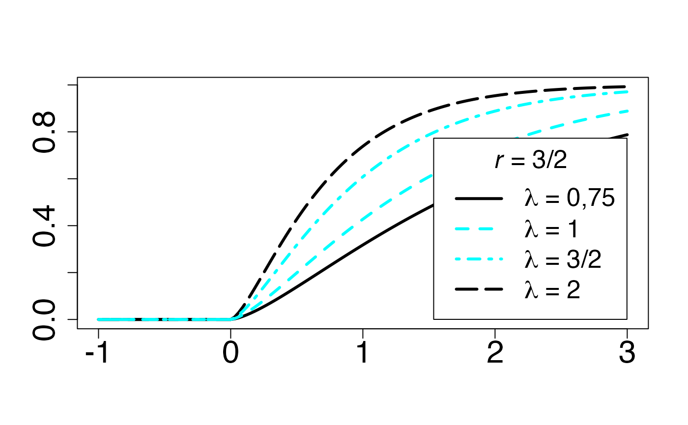
#>       2

Fonction de répartition

Chemin = "~/Documents/Recherche/DeBoeck/Graphes/Fichiers/"
colmodel="cmyk"
pdf(file = paste(Chemin,"frep_",LOI,".pdf",sep=""),
    width = 8, height = 7, onefile = TRUE, family = "Helvetica",
    title = "Probability or cumulative distribution graphs", paper = "special", colormodel = colmodel)
infx=-1;supx=3;
fr <- function(x) {pgamma(x,1.5,2)}
curve(fr,from=infx,to=supx,ylab="",xlab="",lty=1,lwd=3,col=colmagentas[1],type="n",cex.axis=2)
curve(fr,from=infx,to=-0.000001,ylab="",xlab="",lty=5,lwd=3,add=T,col=colmagentas[1])
curve(fr,from=0.000001,to=supx,ylab="",xlab="",lty=5,lwd=3,add=T,col=colmagentas[1])
fr <- function(x) {pgamma(x,1.5,0.75)}
curve(fr,from=infx,to=-0.000001,ylab="",xlab="",lty=1,lwd=3,col=colmagentas[1],add=T)
curve(fr,from=0.000001,to=supx,ylab="",xlab="",lty=1,lwd=3,col=colmagentas[1],add=T)
fr <- function(x) {pgamma(x,1.5,1)}
curve(fr,from=infx,to=-0.000001,ylab="",xlab="",lty=2,lwd=3,add=T,col=colmagentas[2])
curve(fr,from=0.000001,to=supx,ylab="",xlab="",lty=2,lwd=3,add=T,col=colmagentas[2])
fr <- function(x) {pgamma(x,1.5,1.5)}
curve(fr,from=infx,to=-0.000001,ylab="",xlab="",lty=4,lwd=3,add=T,col=colmagentas[3])
curve(fr,from=0.000001,to=supx,ylab="",xlab="",lty=4,lwd=3,add=T,col=colmagentas[3])
leg.txt <- c(expression(paste(lambda," = 0,75",sep="")), expression(paste(lambda," = 1",sep="")), expression(paste(lambda," = 3/2",sep="")),
             expression(paste(lambda," = 2",sep="")))
legend("bottomright", leg.txt, title = expression(paste(italic(r)," = 3/2",sep="")), lty = c(1, 2, 4,5), lwd=3, col = c(colmagentas[1],colmagentas[2],colmagentas[3],colmagentas[1]), cex = 1.6, bg="white", inset=.0375)# , pch = "*"
dev.off()
#> agg_png 
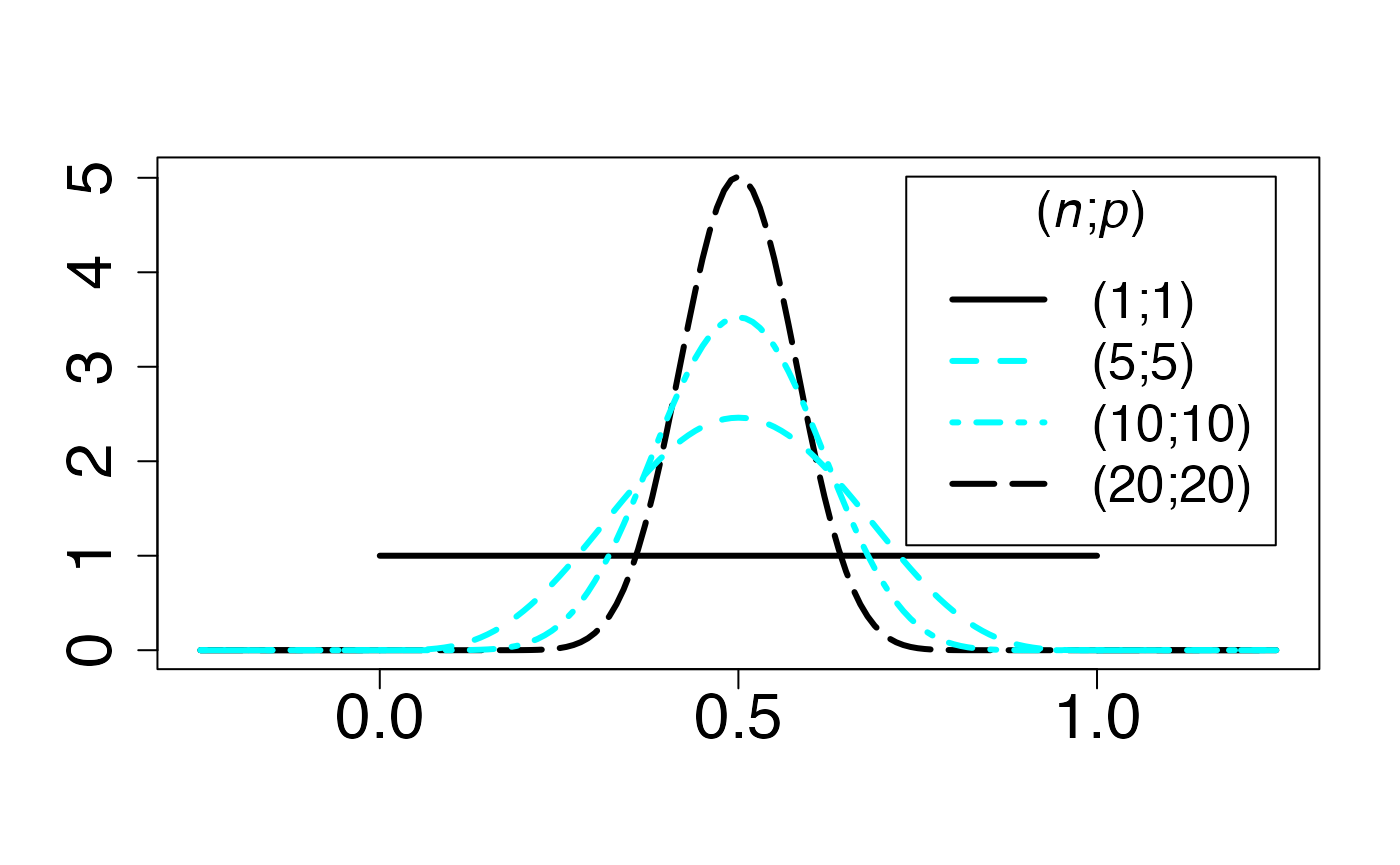
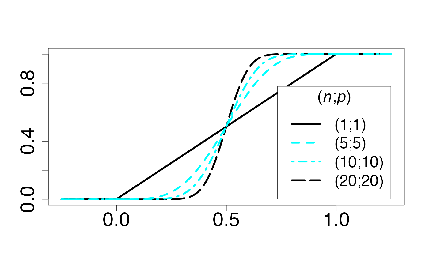
#>       2

Loi bêta (cas uniforme et avec un pic)

Fonction de densité de probabilité

Chemin = "~/Documents/Recherche/DeBoeck/Graphes/Fichiers/"
colmodel="cmyk"
pdf(file = paste(Chemin,"dens_",LOI,".pdf",sep=""),
    width = 8, height = 7, onefile = TRUE, family = "Helvetica",
    title = "Probability or cumulative distribution graphs", paper = "special", colormodel = colmodel)
infx=-0.25;supx=1.25;
fd <- function(x) {dbeta(x,20,20)}
curve(fd,from=infx,to=supx,ylab="",xlab="",lty=1,lwd=3,col=colmagentas[1],type="n",cex.axis=2)
curve(fd,from=infx,to=-0.000001,ylab="",xlab="",lty=5,lwd=3,add=T,col=colmagentas[1])
curve(fd,from=0.000001,to=1.000001,ylab="",xlab="",lty=5,lwd=3,add=T,col=colmagentas[1])
curve(fd,from=1.000001,to=supx,ylab="",xlab="",lty=5,lwd=3,add=T,col=colmagentas[1])
fd <- function(x) {dbeta(x,1,1)}
curve(fd,from=infx,to=-0.000001,ylab="",xlab="",lty=1,lwd=3,col=colmagentas[1],add=T)
curve(fd,from=0.000001,to=0.999999,ylab="",xlab="",lty=1,lwd=3,col=colmagentas[1],add=T)
curve(fd,from=1.000001,to=supx,ylab="",xlab="",lty=1,lwd=3,col=colmagentas[1],add=T)
fd <- function(x) {dbeta(x,5,5)}
curve(fd,from=infx,to=-0.000001,ylab="",xlab="",lty=2,lwd=3,add=T,col=colmagentas[2])
curve(fd,from=0.000001,to=1,ylab="",xlab="",lty=2,lwd=3,add=T,col=colmagentas[2])
curve(fd,from=1,to=supx,ylab="",xlab="",lty=2,lwd=3,add=T,col=colmagentas[2])
fd <- function(x) {dbeta(x,10,10)}
curve(fd,from=infx,to=-0.000001,ylab="",xlab="",lty=4,lwd=3,add=T,col=colmagentas[3])
curve(fd,from=0.000001,to=1,ylab="",xlab="",lty=4,lwd=3,add=T,col=colmagentas[3])
curve(fd,from=1,to=supx,ylab="",xlab="",lty=4,lwd=3,add=T,col=colmagentas[3])
leg.txt <- c("(1;1)", "(5;5)", "(10;10)",
             "(20;20)")
legend("topright", leg.txt, title = expression(paste("(",italic(n),";",italic(p),")",sep="")), lty = c(1, 2, 4,5), lwd=3, col = c(colmagentas[1],colmagentas[2],colmagentas[3],colmagentas[1]), cex = 1.6, bg="white", inset=.0375)# , pch = "*"
dev.off()
#> agg_png 
#>       2

Fonction de répartition

Chemin = "~/Documents/Recherche/DeBoeck/Graphes/Fichiers/"
colmodel="cmyk"
pdf(file = paste(Chemin,"frep_",LOI,".pdf",sep=""),
    width = 8, height = 7, onefile = TRUE, family = "Helvetica",
    title = "Probability or cumulative distribution graphs", paper = "special", colormodel = colmodel)
fr <- function(x) {pbeta(x,20,20)}
curve(fr,from=infx,to=supx,ylab="",xlab="",lty=1,lwd=3,col=colmagentas[1],type="n",cex.axis=2)
curve(fr,from=infx,to=-0.000001,ylab="",xlab="",lty=5,lwd=3,add=T,col=colmagentas[1])
curve(fr,from=0.000001,to=1.000001,ylab="",xlab="",lty=5,lwd=3,add=T,col=colmagentas[1])
curve(fr,from=1.000001,to=supx,ylab="",xlab="",lty=5,lwd=3,add=T,col=colmagentas[1])
fr <- function(x) {pbeta(x,1,1)}
curve(fr,from=infx,to=-0.000001,ylab="",xlab="",lty=1,lwd=3,col=colmagentas[1],add=T)
curve(fr,from=0.000001,to=0.999999,ylab="",xlab="",lty=1,lwd=3,col=colmagentas[1],add=T)
curve(fr,from=1.000001,to=supx,ylab="",xlab="",lty=1,lwd=3,col=colmagentas[1],add=T)
fr <- function(x) {pbeta(x,5,5)}
curve(fr,from=infx,to=-0.000001,ylab="",xlab="",lty=2,lwd=3,add=T,col=colmagentas[2])
curve(fr,from=0.000001,to=1,ylab="",xlab="",lty=2,lwd=3,add=T,col=colmagentas[2])
curve(fr,from=1,to=supx,ylab="",xlab="",lty=2,lwd=3,add=T,col=colmagentas[2])
fr <- function(x) {pbeta(x,10,10)}
curve(fr,from=infx,to=-0.000001,ylab="",xlab="",lty=4,lwd=3,add=T,col=colmagentas[3])
curve(fr,from=0.000001,to=1,ylab="",xlab="",lty=4,lwd=3,add=T,col=colmagentas[3])
curve(fr,from=1,to=supx,ylab="",xlab="",lty=4,lwd=3,add=T,col=colmagentas[3])
leg.txt <- c("(1;1)", "(5;5)", "(10;10)",
             "(20;20)")
legend("bottomright", leg.txt, title = expression(paste("(",italic(n),";",italic(p),")",sep="")), lty = c(1, 2, 4,5), lwd=3, col = c(colmagentas[1],colmagentas[2],colmagentas[3],colmagentas[1]), cex = 1.6, bg="white", inset=.0375)# , pch = "*"
dev.off()
#> agg_png 
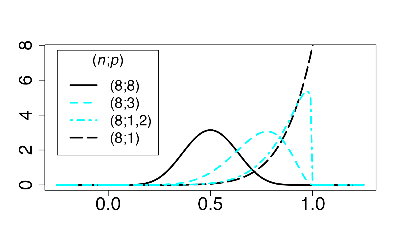
#>       2

Loi bêta (cas asymétrique)

Fonction de densité de probabilité

Chemin = "~/Documents/Recherche/DeBoeck/Graphes/Fichiers/"
colmodel="cmyk"
pdf(file = paste(Chemin,"dens_",LOI,".pdf",sep=""),
    width = 8, height = 7, onefile = TRUE, family = "Helvetica",
    title = "Probability or cumulative distribution graphs", paper = "special", colormodel = colmodel)
infx=-0.25;supx=1.25;
fd <- function(x) {dbeta(x,8,1)}
curve(fd,from=infx,to=supx,ylab="",xlab="",lty=1,lwd=3,col=colmagentas[1],type="n",cex.axis=2)
curve(fd,from=infx,to=-0.000001,ylab="",xlab="",lty=5,lwd=3,add=T,col=colmagentas[1])
curve(fd,from=0.000001,to=0.999999,ylab="",xlab="",lty=5,lwd=3,add=T,col=colmagentas[1])
curve(fd,from=1.000001,to=supx,ylab="",xlab="",lty=5,lwd=3,add=T,col=colmagentas[1])
fd <- function(x) {dbeta(x,8,8)}
curve(fd,from=infx,to=-0.000001,ylab="",xlab="",lty=1,lwd=3,col=colmagentas[1],add=T)
curve(fd,from=0.000001,to=0.999999,ylab="",xlab="",lty=1,lwd=3,col=colmagentas[1],add=T)
curve(fd,from=1.000001,to=supx,ylab="",xlab="",lty=1,lwd=3,col=colmagentas[1],add=T)
fd <- function(x) {dbeta(x,8,3)}
curve(fd,from=infx,to=-0.000001,ylab="",xlab="",lty=2,lwd=3,add=T,col=colmagentas[2])
curve(fd,from=0.000001,to=1,ylab="",xlab="",lty=2,lwd=3,add=T,col=colmagentas[2])
curve(fd,from=1,to=supx,ylab="",xlab="",lty=2,lwd=3,add=T,col=colmagentas[2])
fd <- function(x) {dbeta(x,8,1.2)}
curve(fd,from=infx,to=-0.000001,ylab="",xlab="",lty=4,lwd=3,add=T,col=colmagentas[3])
curve(fd,from=0.000001,to=1,ylab="",xlab="",lty=4,lwd=3,add=T,col=colmagentas[3])
curve(fd,from=1,to=supx,ylab="",xlab="",lty=4,lwd=3,add=T,col=colmagentas[3])
leg.txt <- c("(8;8)", "(8;3)", "(8;1,2)",
             "(8;1)")
legend("topleft", leg.txt, title = expression(paste("(",italic(n),";",italic(p),")",sep="")), lty = c(1, 2, 4,5), lwd=3, col = c(colmagentas[1],colmagentas[2],colmagentas[3],colmagentas[1]), cex = 1.6, bg="white", inset=.0375)# , pch = "*"
dev.off()
#> agg_png 
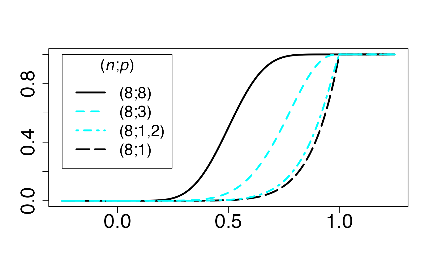
#>       2

Fonction de répartition

Chemin = "~/Documents/Recherche/DeBoeck/Graphes/Fichiers/"
colmodel="cmyk"
pdf(file = paste(Chemin,"frep_",LOI,".pdf",sep=""),
    width = 8, height = 7, onefile = TRUE, family = "Helvetica",
    title = "Probability or cumulative distribution graphs", paper = "special", colormodel = colmodel)
fr <- function(x) {pbeta(x,8,1)}
curve(fr,from=infx,to=supx,ylab="",xlab="",lty=1,lwd=3,col=colmagentas[1],type="n",cex.axis=2)
curve(fr,from=infx,to=-0.000001,ylab="",xlab="",lty=5,lwd=3,add=T,col=colmagentas[1])
curve(fr,from=0.000001,to=0.999999,ylab="",xlab="",lty=5,lwd=3,add=T,col=colmagentas[1])
curve(fr,from=1.000001,to=supx,ylab="",xlab="",lty=5,lwd=3,add=T,col=colmagentas[1])
fr <- function(x) {pbeta(x,8,8)}
curve(fr,from=infx,to=-0.000001,ylab="",xlab="",lty=1,lwd=3,col=colmagentas[1],add=T)
curve(fr,from=0.000001,to=0.999999,ylab="",xlab="",lty=1,lwd=3,col=colmagentas[1],add=T)
curve(fr,from=1.000001,to=supx,ylab="",xlab="",lty=1,lwd=3,col=colmagentas[1],add=T)
fr <- function(x) {pbeta(x,8,3)}
curve(fr,from=infx,to=-0.000001,ylab="",xlab="",lty=2,lwd=3,add=T,col=colmagentas[2])
curve(fr,from=0.000001,to=1,ylab="",xlab="",lty=2,lwd=3,add=T,col=colmagentas[2])
curve(fr,from=1,to=supx,ylab="",xlab="",lty=2,lwd=3,add=T,col=colmagentas[2])
fr <- function(x) {pbeta(x,8,1.2)}
curve(fr,from=infx,to=-0.000001,ylab="",xlab="",lty=4,lwd=3,add=T,col=colmagentas[3])
curve(fr,from=0.000001,to=1,ylab="",xlab="",lty=4,lwd=3,add=T,col=colmagentas[3])
curve(fr,from=1,to=supx,ylab="",xlab="",lty=4,lwd=3,add=T,col=colmagentas[3])
leg.txt <- c("(8;8)", "(8;3)", "(8;1,2)",
             "(8;1)")
legend("topleft", leg.txt, title = expression(paste("(",italic(n),";",italic(p),")",sep="")), lty = c(1, 2, 4,5), lwd=3, col = c(colmagentas[1],colmagentas[2],colmagentas[3],colmagentas[1]), cex = 1.6, bg="white", inset=.0375)# , pch = "*"
dev.off()
#> agg_png 
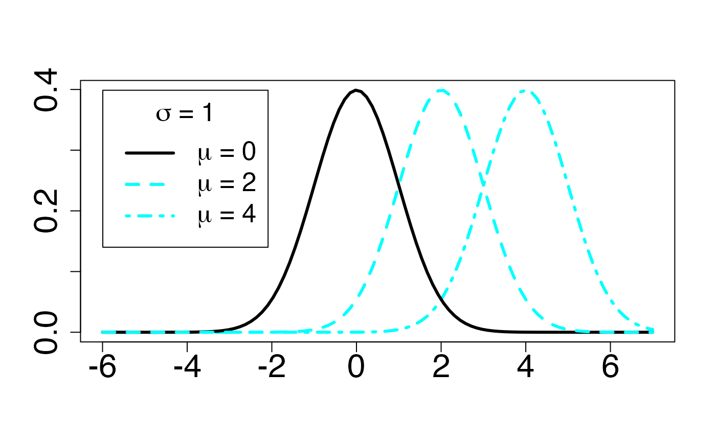
#>       2

Loi de Gauss ou loi normale (en fonction de $\mu$)

Fonction de densité de probabilité

Chemin = "~/Documents/Recherche/DeBoeck/Graphes/Fichiers/"
colmodel="cmyk"
pdf(file = paste(Chemin,"dens_",LOI,".pdf",sep=""),
    width = 8, height = 7, onefile = TRUE, family = "Helvetica",
    title = "Probability or cumulative distribution graphs", paper = "special", colormodel = colmodel)
infx=-6;supx=7;
fd <- function(x) {dnorm(x,4,1)}
curve(fd,from=infx,to=supx,ylab="",xlab="",lty=1,lwd=3,col=colmagentas[1],type="n",cex.axis=2)
curve(fd,from=infx,to=supx,ylab="",xlab="",lty=4,lwd=3,add=T,col=colmagentas[3])
fd <- function(x) {dnorm(x,0,1)}
curve(fd,from=infx,to=supx,ylab="",xlab="",lty=1,lwd=3,col=colmagentas[1],add=T)
fd <- function(x) {dnorm(x,2,1)}
curve(fd,from=infx,to=supx,ylab="",xlab="",lty=2,lwd=3,add=T,col=colmagentas[2])
leg.txt <- c(expression(paste(mu," = 0",sep="")), expression(paste(mu," = 2",sep="")), expression(paste(mu," = 4",sep="")))
legend("topleft", leg.txt, title = expression(paste(sigma," = 1",sep="")), lty = c(1, 2, 4), lwd=3, col = c(colmagentas[1],colmagentas[2],colmagentas[3]), cex = 1.6, bg="white", inset=.0375)# , pch = "*"
dev.off()
#> agg_png 
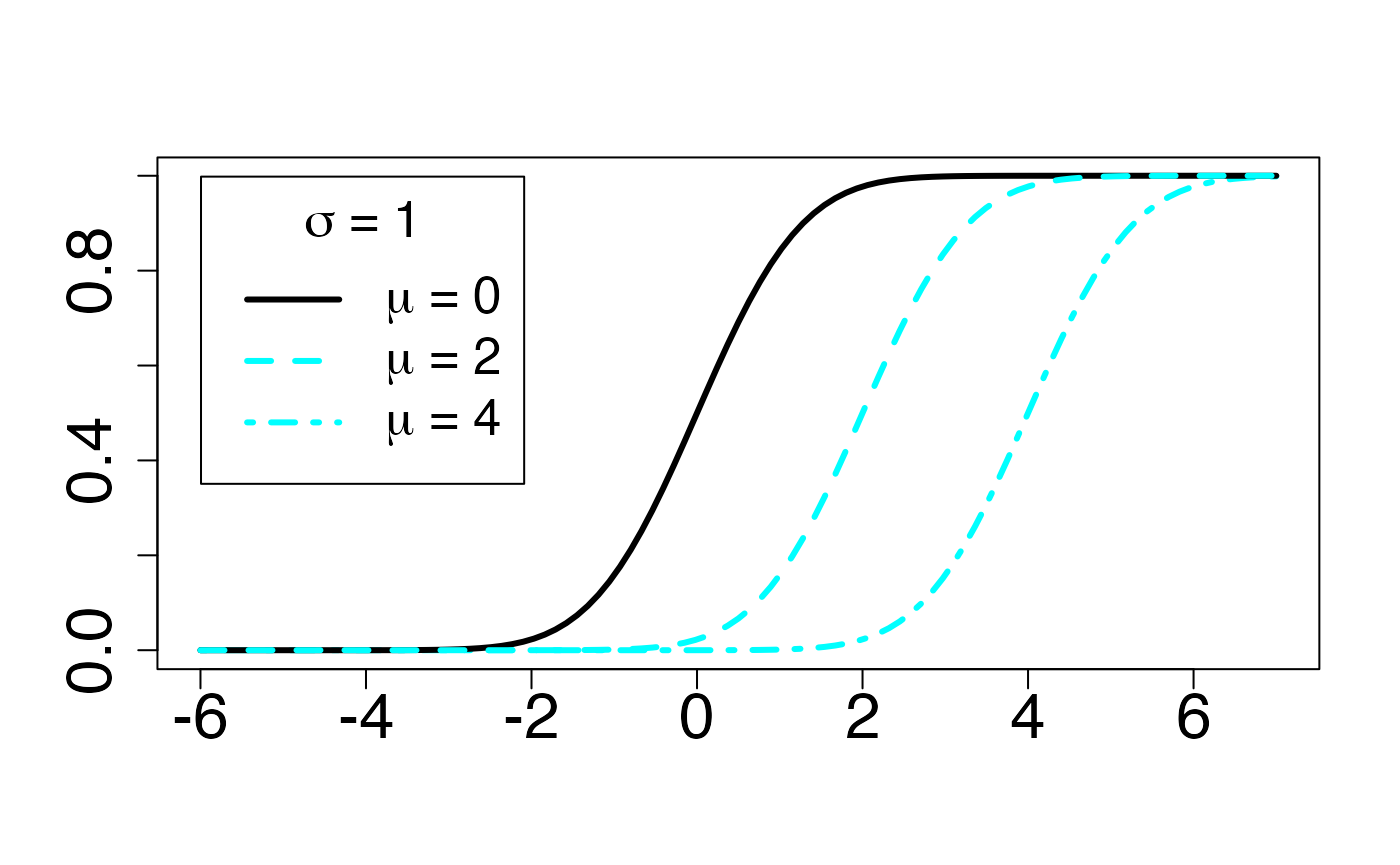
#>       2

Fonction de répartition

Chemin = "~/Documents/Recherche/DeBoeck/Graphes/Fichiers/"
colmodel="cmyk"
pdf(file = paste(Chemin,"frep_",LOI,".pdf",sep=""),
    width = 8, height = 7, onefile = TRUE, family = "Helvetica",
    title = "Probability or cumulative distribution graphs", paper = "special", colormodel = colmodel)
infx=-6;supx=7;
fr <- function(x) {pnorm(x,4,1)}
curve(fr,from=infx,to=supx,ylab="",xlab="",lty=1,lwd=3,col=colmagentas[1],type="n",cex.axis=2)
curve(fr,from=infx,to=supx,ylab="",xlab="",lty=4,lwd=3,add=T,col=colmagentas[3])
fr <- function(x) {pnorm(x,0,1)}
curve(fr,from=infx,to=supx,ylab="",xlab="",lty=1,lwd=3,col=colmagentas[1],add=T)
fr <- function(x) {pnorm(x,2,1)}
curve(fr,from=infx,to=supx,ylab="",xlab="",lty=2,lwd=3,add=T,col=colmagentas[2])
leg.txt <- c(expression(paste(mu," = 0",sep="")), expression(paste(mu," = 2",sep="")), expression(paste(mu," = 4",sep="")))
legend("topleft", leg.txt, title = expression(paste(sigma," = 1",sep="")), lty = c(1, 2, 4), lwd=3, col = c(colmagentas[1],colmagentas[2],colmagentas[3]), cex = 1.6, bg="white", inset=.0375)# , pch = "*"
dev.off()
#> agg_png 
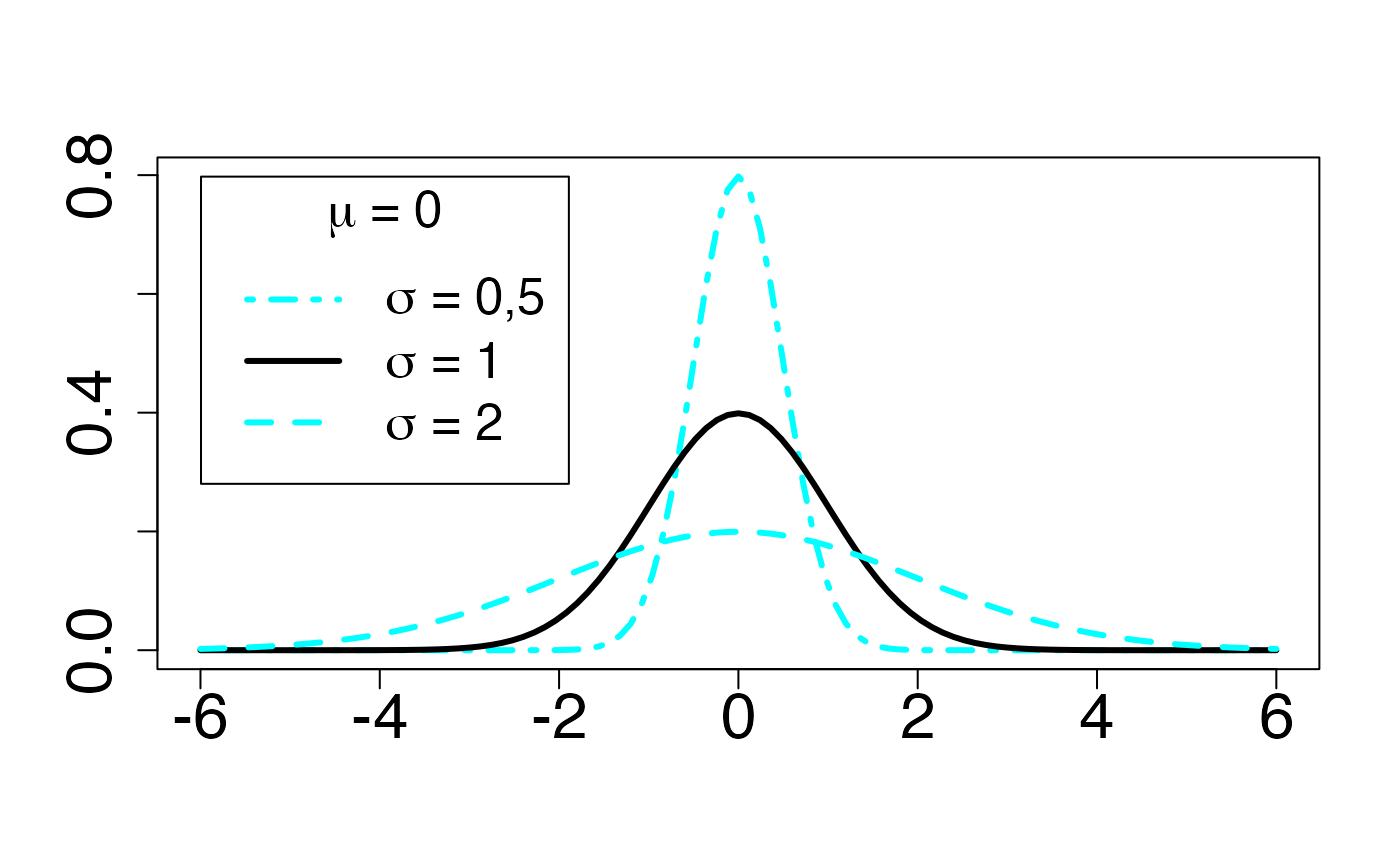
#>       2

Loi de Gauss ou loi normale (en fonction de $\sigma$)

Fonction de densité de probabilité

Chemin = "~/Documents/Recherche/DeBoeck/Graphes/Fichiers/"
colmodel="cmyk"
pdf(file = paste(Chemin,"dens_",LOI,".pdf",sep=""),
    width = 8, height = 7, onefile = TRUE, family = "Helvetica",
    title = "Probability or cumulative distribution graphs", paper = "special", colormodel = colmodel)
infx=-6;supx=6;
fd <- function(x) {dnorm(x,0,1/2)}
curve(fd,from=infx,to=supx,ylab="",xlab="",lty=1,lwd=3,col=colmagentas[1],type="n",cex.axis=2)
curve(fd,from=infx,to=supx,ylab="",xlab="",lty=4,lwd=3,add=T,col=colmagentas[3])
fd <- function(x) {dnorm(x,0,1)}
curve(fd,from=infx,to=supx,ylab="",xlab="",lty=1,lwd=3,col=colmagentas[1],add=T)
fd <- function(x) {dnorm(x,0,2)}
curve(fd,from=infx,to=supx,ylab="",xlab="",lty=2,lwd=3,add=T,col=colmagentas[2])
leg.txt <- c(expression(paste(sigma," = 0,5",sep="")), expression(paste(sigma," = 1",sep="")), expression(paste(sigma," = 2",sep="")))
legend("topleft", leg.txt, title = expression(paste(mu, " = 0", sep="")), lty = c(4, 1, 2), lwd=3, col = c(colmagentas[3],colmagentas[1],colmagentas[2]), cex = 1.6, bg="white", inset=.0375)# , pch = "*"
dev.off()
#> agg_png 
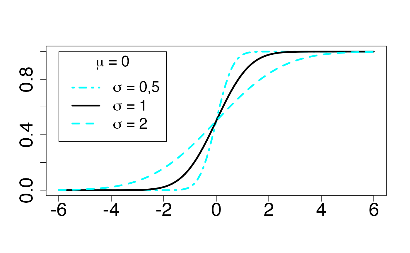
#>       2

Fonction de répartition

Chemin = "~/Documents/Recherche/DeBoeck/Graphes/Fichiers/"
colmodel="cmyk"
pdf(file = paste(Chemin,"frep_",LOI,".pdf",sep=""),
    width = 8, height = 7, onefile = TRUE, family = "Helvetica",
    title = "Probability or cumulative distribution graphs", paper = "special", colormodel = colmodel)
infx=-6;supx=6;
fr <- function(x) {pnorm(x,0,1/2)}
curve(fr,from=infx,to=supx,ylab="",xlab="",lty=1,lwd=3,col=colmagentas[1],type="n",cex.axis=2)
curve(fr,from=infx,to=supx,ylab="",xlab="",lty=4,lwd=3,add=T,col=colmagentas[3])
fr <- function(x) {pnorm(x,0,1)}
curve(fr,from=infx,to=supx,ylab="",xlab="",lty=1,lwd=3,col=colmagentas[1],add=T)
fr <- function(x) {pnorm(x,0,2)}
curve(fr,from=infx,to=supx,ylab="",xlab="",lty=2,lwd=3,add=T,col=colmagentas[2])
leg.txt <- c(expression(paste(sigma," = 0,5",sep="")), expression(paste(sigma," = 1",sep="")), expression(paste(sigma," = 2",sep="")))
legend("topleft", leg.txt, title = expression(paste(mu, " = 0", sep="")), lty = c(4, 1, 2), lwd=3, col = c(colmagentas[3],colmagentas[1],colmagentas[2]), cex = 1.6, bg="white", inset=.0375)# , pch = "*"
dev.off()
#> agg_png 
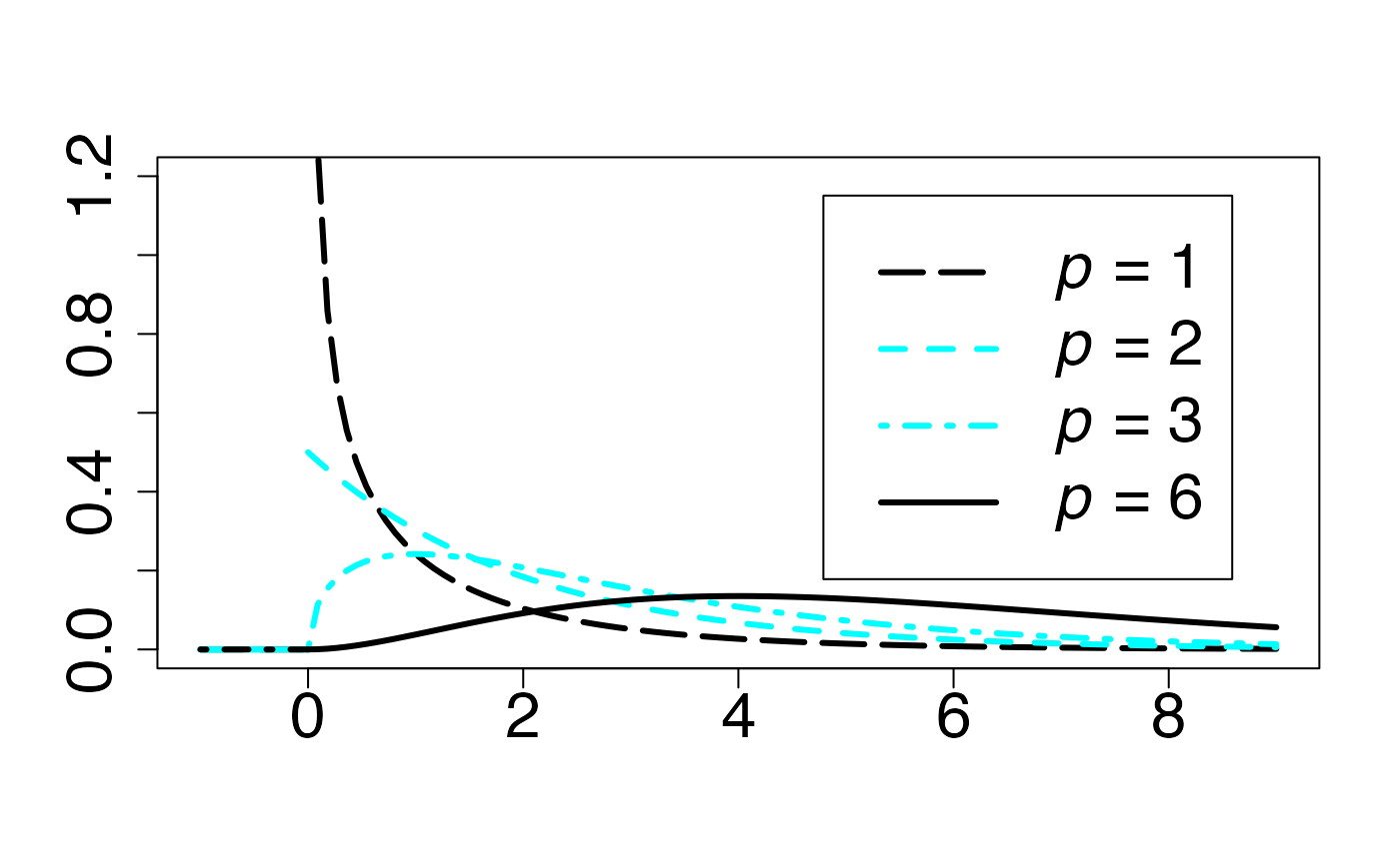
#>       2

Loi du chi-deux (en fonction de $r$)

Fonction de densité de probabilité

Chemin = "~/Documents/Recherche/DeBoeck/Graphes/Fichiers/"
colmodel="cmyk"
pdf(file = paste(Chemin,"dens_",LOI,".pdf",sep=""),
    width = 8, height = 7, onefile = TRUE, family = "Helvetica",
    title = "Probability or cumulative distribution graphs", paper = "special", colormodel = colmodel)
infx=-1;supx=9;
fd <- function(x) {dchisq(x,1)}
curve(fd,from=infx,to=supx,ylab="",xlab="",lty=1,lwd=3,col=colmagentas[1],type="n",cex.axis=2)
curve(fd,from=infx,to=-0.000001,ylab="",xlab="",lty=5,lwd=3,add=T,col=colmagentas[1])
curve(fd,from=0.000001,to=supx,ylab="",xlab="",lty=5,lwd=3,add=T,col=colmagentas[1])
fd <- function(x) {dchisq(x,3)}
curve(fd,from=infx,to=-0.000001,ylab="",xlab="",lty=1,lwd=3,col=colmagentas[3],add=T)
curve(fd,from=0.000001,to=supx,ylab="",xlab="",lty=4,lwd=3,col=colmagentas[3],add=T)
fd <- function(x) {dchisq(x,2)}
curve(fd,from=infx,to=-0.000001,ylab="",xlab="",lty=2,lwd=3,add=T,col=colmagentas[2])
curve(fd,from=0.000001,to=supx,ylab="",xlab="",lty=2,lwd=3,add=T,col=colmagentas[2])
fd <- function(x) {dchisq(x,6)}
curve(fd,from=infx,to=-0.000001,ylab="",xlab="",lty=4,lwd=3,add=T,col=colmagentas[1])
curve(fd,from=0.000001,to=supx,ylab="",xlab="",lty=1,lwd=3,add=T,col=colmagentas[1])
leg.txt <- c(expression(paste(italic(p)," = 1",sep="")), expression(paste(italic(p)," = 2",sep="")), expression(paste(italic(p)," = 3",sep="")),
             expression(paste(italic(p)," = 6",sep="")))
legend("topright", leg.txt, lty = c(5, 2, 4,1), lwd=3, col = c(colmagentas[1],colmagentas[2],colmagentas[3],colmagentas[1]), cex = 2, bg="white", inset=.075)# , pch = "*"
dev.off()
#> agg_png 
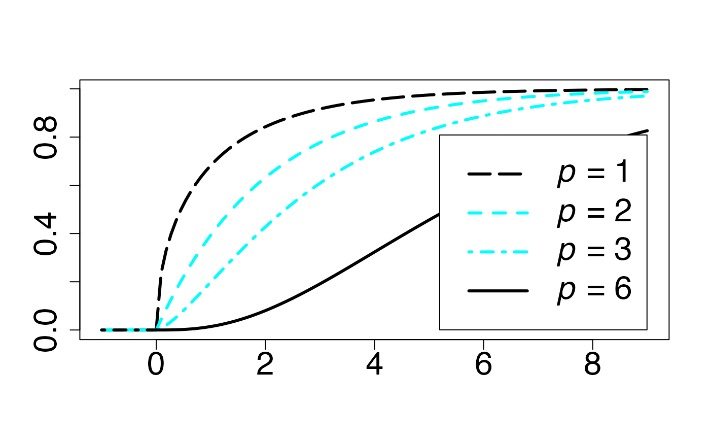
#>       2

Fonction de répartition

Chemin = "~/Documents/Recherche/DeBoeck/Graphes/Fichiers/"
colmodel="cmyk"
pdf(file = paste(Chemin,"frep_",LOI,".pdf",sep=""),
    width = 8, height = 7, onefile = TRUE, family = "Helvetica",
    title = "Probability or cumulative distribution graphs", paper = "special", colormodel = colmodel)
infx=-1;supx=9;
fr <- function(x) {pchisq(x,1)}
curve(fr,from=infx,to=supx,ylab="",xlab="",lty=1,lwd=3,col=colmagentas[1],type="n",cex.axis=2)
curve(fr,from=infx,to=-0.000001,ylab="",xlab="",lty=5,lwd=3,add=T,col=colmagentas[1])
curve(fr,from=0.000001,to=supx,ylab="",xlab="",lty=5,lwd=3,add=T,col=colmagentas[1])
fr <- function(x) {pchisq(x,3)}
curve(fr,from=infx,to=-0.000001,ylab="",xlab="",lty=1,lwd=3,col=colmagentas[3],add=T)
curve(fr,from=0.000001,to=supx,ylab="",xlab="",lty=4,lwd=3,col=colmagentas[3],add=T)
fr <- function(x) {pchisq(x,2)}
curve(fr,from=infx,to=-0.000001,ylab="",xlab="",lty=2,lwd=3,add=T,col=colmagentas[2])
curve(fr,from=0.000001,to=supx,ylab="",xlab="",lty=2,lwd=3,add=T,col=colmagentas[2])
fr <- function(x) {pchisq(x,6)}
curve(fr,from=infx,to=-0.000001,ylab="",xlab="",lty=4,lwd=3,add=T,col=colmagentas[1])
curve(fr,from=0.000001,to=supx,ylab="",xlab="",lty=1,lwd=3,add=T,col=colmagentas[1])
leg.txt <- c(expression(paste(italic(p)," = 1",sep="")), expression(paste(italic(p)," = 2",sep="")), expression(paste(italic(p)," = 3",sep="")),
             expression(paste(italic(p)," = 6",sep="")))
legend("bottomright", leg.txt, lty = c(5, 2, 4,1), lwd=3, col = c(colmagentas[1],colmagentas[2],colmagentas[3],colmagentas[1]), cex = 2, bg="white", inset=.0375)# , pch = "*"
dev.off()
#> agg_png 
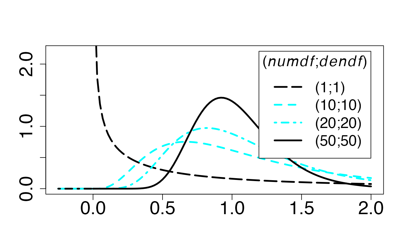
#>       2

Loi de Fisher (cas symétrique)

Fonction de densité de probabilité

Chemin = "~/Documents/Recherche/DeBoeck/Graphes/Fichiers/"
colmodel="cmyk"
pdf(file = paste(Chemin,"dens_",LOI,".pdf",sep=""),
    width = 8, height = 7, onefile = TRUE, family = "Helvetica",
    title = "Probability or cumulative distribution graphs", paper = "special", colormodel = colmodel)
infx=-0.25;supx=2;
fd <- function(x) {df(x,1,1)}
curve(fd,from=infx,to=supx,ylab="",xlab="",lty=1,lwd=3,col=colmagentas[1],type="n",cex.axis=2)
curve(fd,from=infx,to=-0.000001,ylab="",xlab="",lty=1,lwd=3,add=T,col=colmagentas[1])
curve(fd,from=0.01,to=supx,ylab="",xlab="",lty=5,lwd=3,add=T,col=colmagentas[1])
fd <- function(x) {df(x,20,20)}
curve(fd,from=infx,to=-0.000001,ylab="",xlab="",lty=1,lwd=3,col=colmagentas[3],add=T)
curve(fd,from=0.000001,to=supx,ylab="",xlab="",lty=4,lwd=3,col=colmagentas[3],add=T)
fd <- function(x) {df(x,10,10)}
curve(fd,from=infx,to=-0.000001,ylab="",xlab="",lty=2,lwd=3,add=T,col=colmagentas[2])
curve(fd,from=0.000001,to=supx,ylab="",xlab="",lty=2,lwd=3,add=T,col=colmagentas[2])
fd <- function(x) {df(x,50,50)}
curve(fd,from=infx,to=-0.000001,ylab="",xlab="",lty=4,lwd=3,add=T,col=colmagentas[1])
curve(fd,from=0.000001,to=supx,ylab="",xlab="",lty=1,lwd=3,add=T,col=colmagentas[1])
leg.txt <- c("(1;1)", "(10;10)", "(20;20)",
             "(50;50)")
legend("topright", leg.txt, title=expression(paste("(",italic(numdf),";",italic(dendf),")",sep="")), lty = c(5, 2, 4,1), lwd=3, col = c(colmagentas[1],colmagentas[2],colmagentas[3],colmagentas[1]), cex = 1.6, bg="white", inset=.0375)# , pch = "*"
dev.off()
#> agg_png 
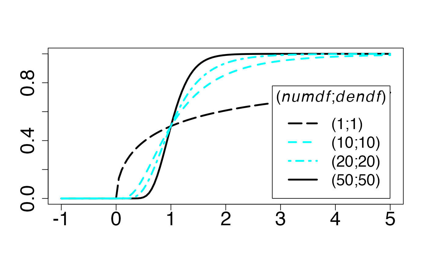
#>       2

Fonction de répartition

Chemin = "~/Documents/Recherche/DeBoeck/Graphes/Fichiers/"
colmodel="cmyk"
pdf(file = paste(Chemin,"frep_",LOI,".pdf",sep=""),
    width = 8, height = 7, onefile = TRUE, family = "Helvetica",
    title = "Probability or cumulative distribution graphs", paper = "special", colormodel = colmodel)
infx=-1;supx=5;
fr <- function(x) {pf(x,50,50)}
curve(fr,from=infx,to=supx,ylab="",xlab="",lty=1,lwd=3,col=colmagentas[1],type="n",cex.axis=2)
curve(fr,from=infx,to=-0.000001,ylab="",xlab="",lty=4,lwd=3,add=T,col=colmagentas[1])
curve(fr,from=0.000001,to=supx,ylab="",xlab="",lty=1,lwd=3,add=T,col=colmagentas[1])
fr <- function(x) {pf(x,1,1)}
curve(fr,from=infx,to=-0.000001,ylab="",xlab="",lty=1,lwd=3,add=T,col=colmagentas[1])
curve(fr,from=0.00001,to=supx,ylab="",xlab="",lty=5,lwd=3,add=T,col=colmagentas[1])
fr <- function(x) {pf(x,20,20)}
curve(fr,from=infx,to=-0.000001,ylab="",xlab="",lty=1,lwd=3,col=colmagentas[3],add=T)
curve(fr,from=0.000001,to=supx,ylab="",xlab="",lty=4,lwd=3,col=colmagentas[3],add=T)
fr <- function(x) {pf(x,10,10)}
curve(fr,from=infx,to=-0.000001,ylab="",xlab="",lty=2,lwd=3,add=T,col=colmagentas[2])
curve(fr,from=0.000001,to=supx,ylab="",xlab="",lty=2,lwd=3,add=T,col=colmagentas[2])
leg.txt <- c("(1;1)", "(10;10)", "(20;20)",
             "(50;50)")
legend("bottomright", leg.txt, title=expression(paste("(",italic(numdf),";",italic(dendf),")",sep="")), lty = c(5, 2, 4,1), lwd=3, col = c(colmagentas[1],colmagentas[2],colmagentas[3],colmagentas[1]), cex = 1.6, bg="white", inset=.0375)# , pch = "*"
dev.off()
#> agg_png 
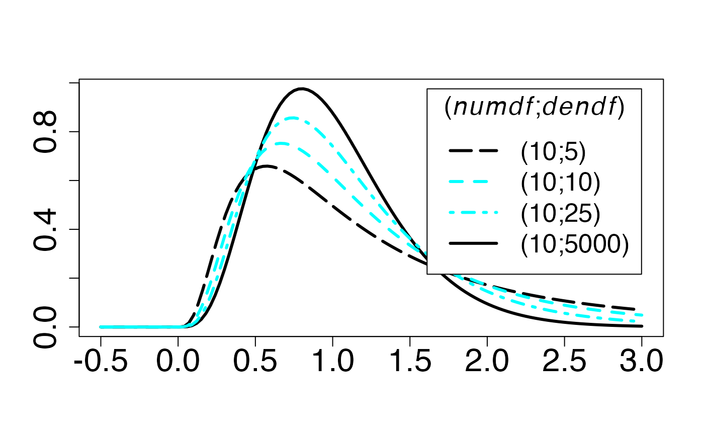
#>       2

Loi de Fisher (cas asymétrique)

Fonction de densité de probabilité

Chemin = "~/Documents/Recherche/DeBoeck/Graphes/Fichiers/"
colmodel="cmyk"
pdf(file = paste(Chemin,"dens_",LOI,".pdf",sep=""),
    width = 8, height = 7, onefile = TRUE, family = "Helvetica",
    title = "Probability or cumulative distribution graphs", paper = "special", colormodel = colmodel)
infx=-0.5;supx=3;
fd <- function(x) {df(x,10,5000)}
curve(fd,from=infx,to=supx,ylab="",xlab="",lty=1,lwd=3,col=colmagentas[1],type="n",cex.axis=2)
curve(fd,from=infx,to=-0.000001,ylab="",xlab="",lty=4,lwd=3,add=T,col=colmagentas[1])
curve(fd,from=0.000001,to=supx,ylab="",xlab="",lty=1,lwd=3,add=T,col=colmagentas[1])
fd <- function(x) {df(x,10,5)}
curve(fd,from=infx,to=-0.000001,ylab="",xlab="",lty=1,lwd=3,add=T,col=colmagentas[1])
curve(fd,from=0.01,to=supx,ylab="",xlab="",lty=5,lwd=3,add=T,col=colmagentas[1])
fd <- function(x) {df(x,10,10)}
curve(fd,from=infx,to=-0.000001,ylab="",xlab="",lty=1,lwd=3,col=colmagentas[2],add=T)
curve(fd,from=0.000001,to=supx,ylab="",xlab="",lty=2,lwd=3,col=colmagentas[2],add=T)
fd <- function(x) {df(x,10,25)}
curve(fd,from=infx,to=-0.000001,ylab="",xlab="",lty=2,lwd=3,add=T,col=colmagentas[3])
curve(fd,from=0.000001,to=supx,ylab="",xlab="",lty=4,lwd=3,add=T,col=colmagentas[3])
leg.txt <- c("(10;5)", "(10;10)", "(10;25)",
             "(10;5000)")
legend("topright", leg.txt, title=expression(paste("(",italic(numdf),";",italic(dendf),")",sep="")), lty = c(5, 2, 4,1), lwd=3, col = c(colmagentas[1],colmagentas[2],colmagentas[3],colmagentas[1]), cex = 1.6, bg="white", inset=.0375)# , pch = "*"
dev.off()
#> agg_png 
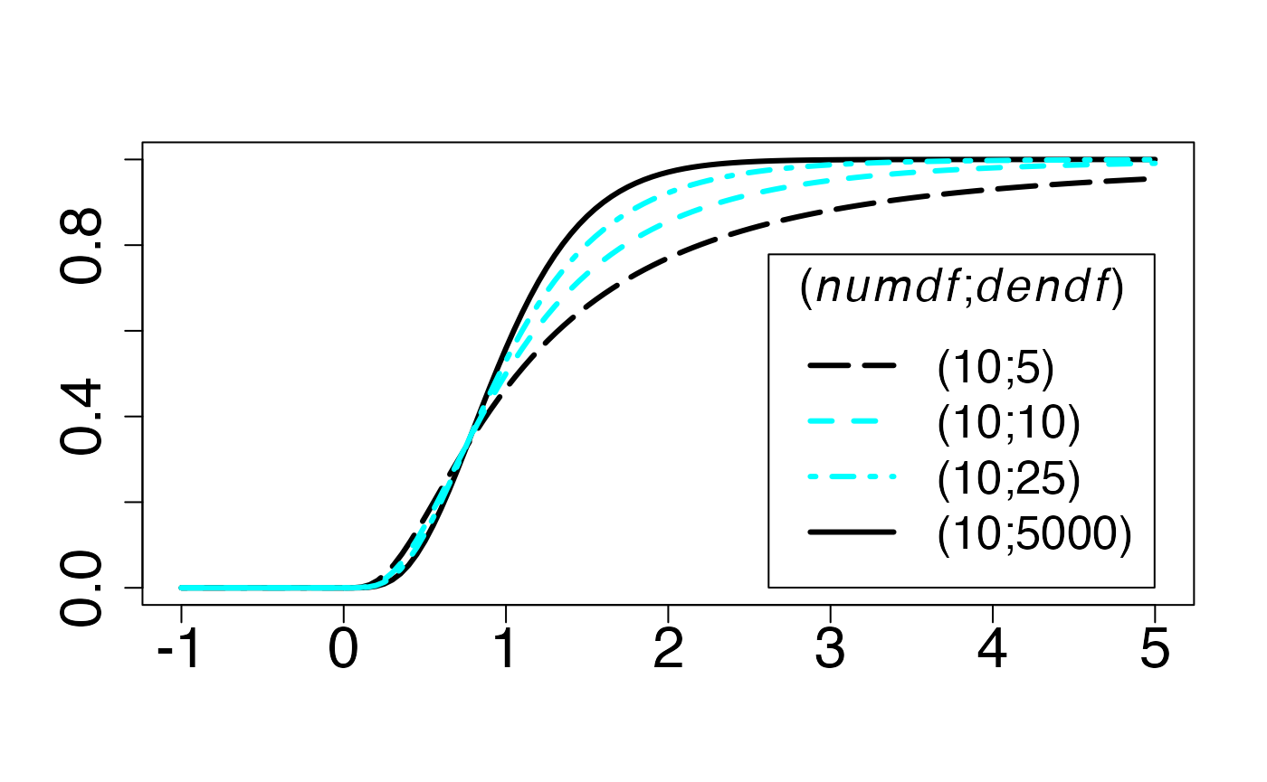
#>       2

Fonction de répartition

Chemin = "~/Documents/Recherche/DeBoeck/Graphes/Fichiers/"
colmodel="cmyk"
pdf(file = paste(Chemin,"frep_",LOI,".pdf",sep=""),
    width = 8, height = 7, onefile = TRUE, family = "Helvetica",
    title = "Probability or cumulative distribution graphs", paper = "special", colormodel = colmodel)
infx=-1;supx=5;
fr <- function(x) {pf(x,10,5000)}
curve(fr,from=infx,to=supx,ylab="",xlab="",lty=1,lwd=3,col=colmagentas[1],type="n",cex.axis=2)
curve(fr,from=infx,to=-0.000001,ylab="",xlab="",lty=4,lwd=3,add=T,col=colmagentas[1])
curve(fr,from=0.000001,to=supx,ylab="",xlab="",lty=1,lwd=3,add=T,col=colmagentas[1])
fr <- function(x) {pf(x,10,5)}
curve(fr,from=infx,to=-0.000001,ylab="",xlab="",lty=1,lwd=3,add=T,col=colmagentas[1])
curve(fr,from=0.01,to=supx,ylab="",xlab="",lty=5,lwd=3,add=T,col=colmagentas[1])
fr <- function(x) {pf(x,10,10)}
curve(fr,from=infx,to=-0.000001,ylab="",xlab="",lty=1,lwd=3,col=colmagentas[2],add=T)
curve(fr,from=0.000001,to=supx,ylab="",xlab="",lty=2,lwd=3,col=colmagentas[2],add=T)
fr <- function(x) {pf(x,10,25)}
curve(fr,from=infx,to=-0.000001,ylab="",xlab="",lty=2,lwd=3,add=T,col=colmagentas[3])
curve(fr,from=0.000001,to=supx,ylab="",xlab="",lty=4,lwd=3,add=T,col=colmagentas[3])
leg.txt <- c("(10;5)", "(10;10)", "(10;25)",
             "(10;5000)")
legend("bottomright", leg.txt, title=expression(paste("(",italic(numdf),";",italic(dendf),")",sep="")), lty = c(5, 2, 4,1), lwd=3, col = c(colmagentas[1],colmagentas[2],colmagentas[3],colmagentas[1]), cex = 1.6, bg="white", inset=.0375)# , pch = "*"
dev.off()
#> agg_png 
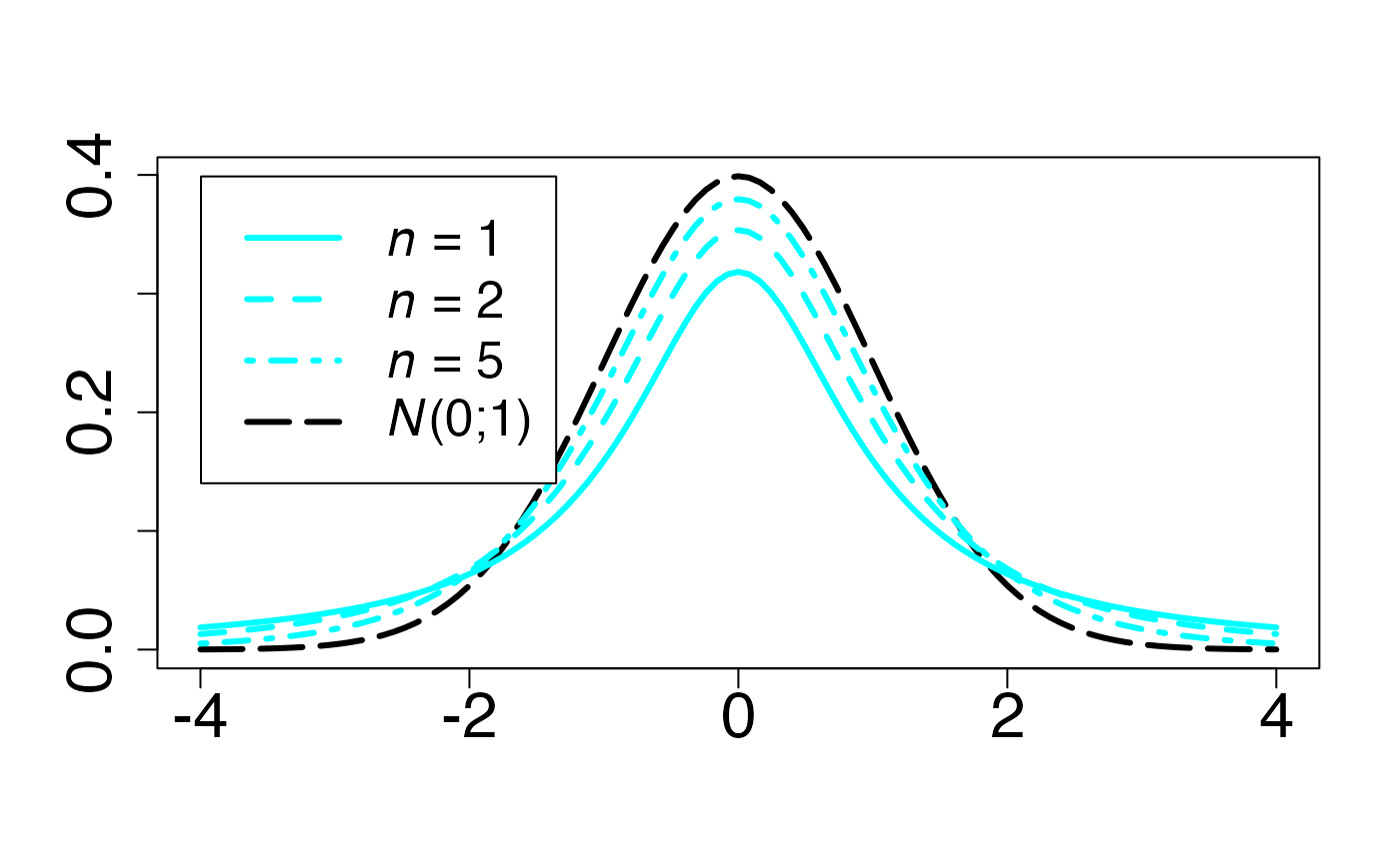
#>       2

Loi de student (en fonction de $n$)

Fonction de densité de probabilité

Chemin = "~/Documents/Recherche/DeBoeck/Graphes/Fichiers/"
colmodel="cmyk"
pdf(file = paste(Chemin,"dens_",LOI,".pdf",sep=""),
    width = 8, height = 7, onefile = TRUE, family = "Helvetica",
    title = "Probability or cumulative distribution graphs", paper = "special", colormodel = colmodel)
LOI <- "student"
infx=-4;supx=4;
fd <- function(x) {dnorm(x)}
curve(fd,from=infx,to=supx,ylab="",xlab="",lty=5,lwd=3,add=F,col=colmagentas[1],cex.axis=2)
fd <- function(x) {dt(x,1)}
curve(fd,from=infx,to=supx,ylab="",xlab="",lty=1,lwd=3,add=T,col=colmagentas[2])
fd <- function(x) {dt(x,2)}
curve(fd,from=infx,to=supx,ylab="",xlab="",lty=2,lwd=3,add=T,col=colmagentas[3])
fd <- function(x) {dt(x,5)}
curve(fd,from=infx,to=supx,ylab="",xlab="",lty=4,lwd=3,add=T,col=colmagentas[4])
leg.txt <- c(expression(paste(italic(n)," = 1",sep="")), expression(paste(italic(n)," = 2",sep="")), expression(paste(italic(n)," = 5",sep="")),
             expression(paste(italic(N),"(0;1)",sep="")))
legend("topleft", leg.txt, lty = c(1, 2, 4,5), lwd=3, col = c(colmagentas[2],colmagentas[3],colmagentas[4],colmagentas[1]), cex = 1.6, bg="white", inset=.0375)# , pch = "*"
dev.off()
#> agg_png 
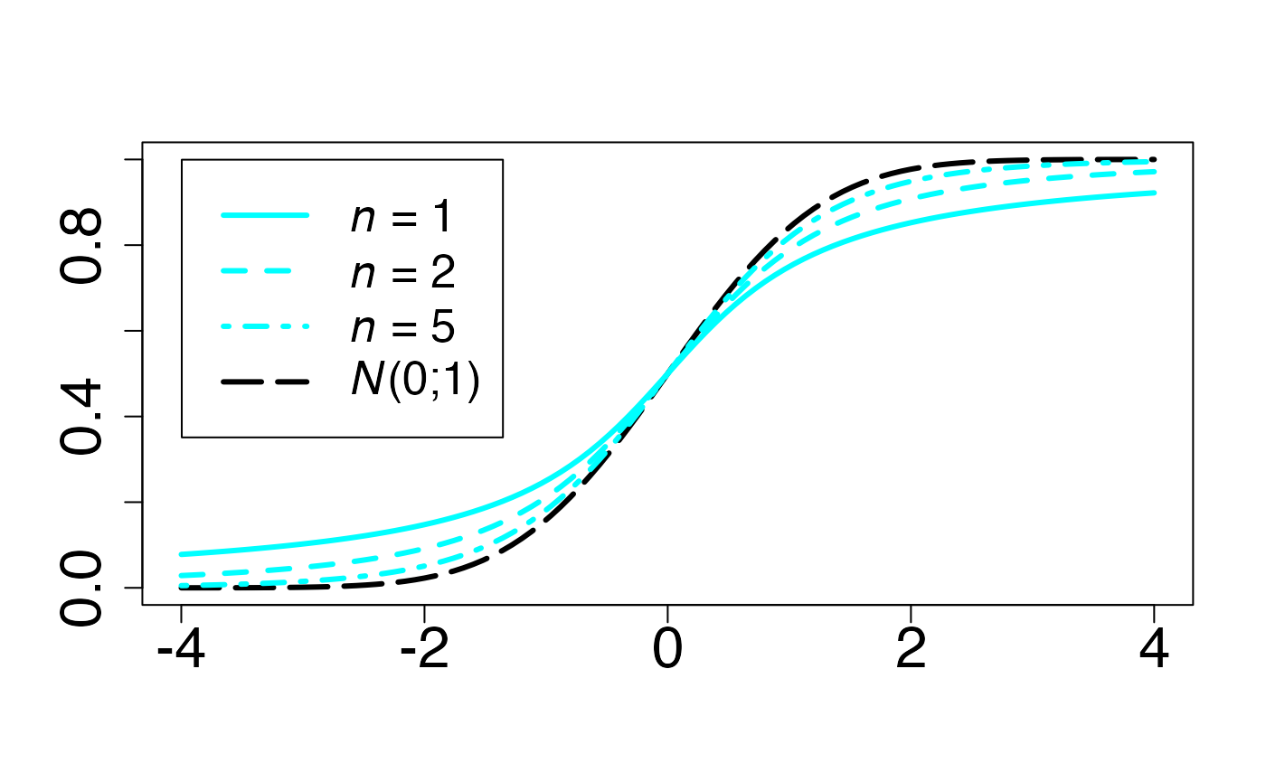
#>       2

Fonction de répartition

Chemin = "~/Documents/Recherche/DeBoeck/Graphes/Fichiers/"
colmodel="cmyk"
pdf(file = paste(Chemin,"frep_",LOI,".pdf",sep=""),
    width = 8, height = 7, onefile = TRUE, family = "Helvetica",
    title = "Probability or cumulative distribution graphs", paper = "special", colormodel = colmodel)
infx=-4;supx=4;
fr <- function(x) {pnorm(x)}
curve(fr,from=infx,to=supx,ylab="",xlab="",lty=5,lwd=3,add=F,col=colmagentas[1],cex.axis=2)
fr <- function(x) {pt(x,1)}
curve(fr,from=infx,to=supx,ylab="",xlab="",lty=1,lwd=3,add=T,col=colmagentas[2])
fr <- function(x) {pt(x,2)}
curve(fr,from=infx,to=supx,ylab="",xlab="",lty=2,lwd=3,add=T,col=colmagentas[3])
fr <- function(x) {pt(x,5)}
curve(fr,from=infx,to=supx,ylab="",xlab="",lty=4,lwd=3,add=T,col=colmagentas[4])
leg.txt <- c(expression(paste(italic(n)," = 1",sep="")), expression(paste(italic(n)," = 2",sep="")), expression(paste(italic(n)," = 5",sep="")),
             expression(paste(italic(N),"(0;1)",sep="")))
legend("topleft", leg.txt, lty = c(1, 2, 4,5), lwd=3, col = c(colmagentas[2],colmagentas[3],colmagentas[4],colmagentas[1]), cex = 1.6, bg="white", inset=.0375)# , pch = "*"
dev.off()
#> agg_png 
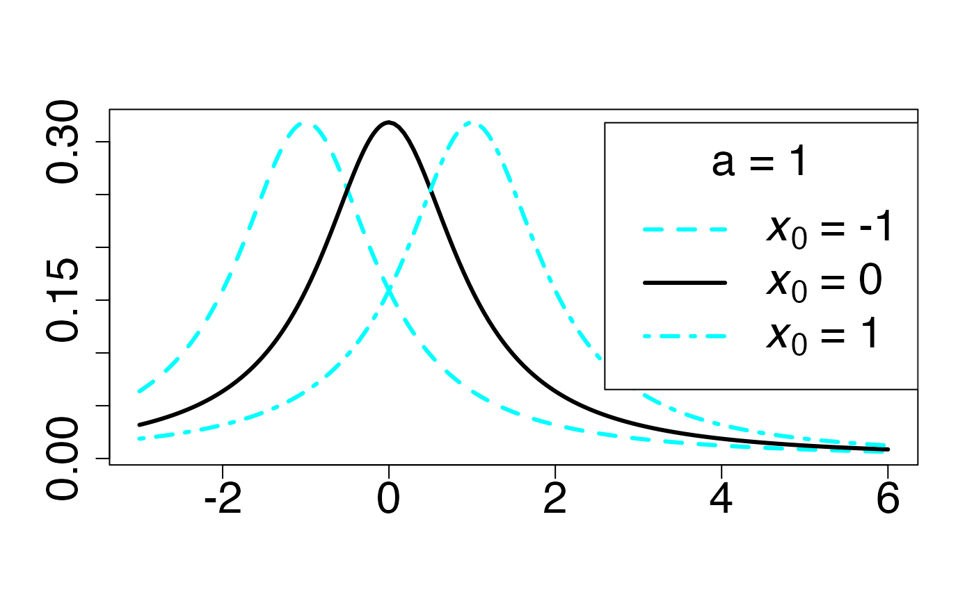
#>       2

Loi de Cauchy (en fonction de $x$)

Fonction de densité de probabilité

Chemin = "~/Documents/Recherche/DeBoeck/Graphes/Fichiers/"
colmodel="cmyk"
pdf(file = paste(Chemin,"dens_",LOI,".pdf",sep=""),
    width = 8, height = 7, onefile = TRUE, family = "Helvetica",
    title = "Probability or cumulative distribution graphs", paper = "special", colormodel = colmodel)
infx=-3;supx=6;
fd <- function(x) {dcauchy(x,-1)}
curve(fd,from=infx,to=supx,ylab="",xlab="",lty=1,lwd=3,col=colmagentas[1],type="n",cex.axis=2)
curve(fd,from=infx,to=-0.000001,ylab="",xlab="",lty=2,lwd=3,col=colmagentas[2],add=T)
curve(fd,from=0.000001,to=supx,ylab="",xlab="",lty=2,lwd=3,col=colmagentas[2],add=T)
fd <- function(x) {dcauchy(x,0)}
curve(fd,from=infx,to=-0.000001,ylab="",xlab="",lty=1,lwd=3,add=T,col=colmagentas[1])
curve(fd,from=0.000001,to=supx,ylab="",xlab="",lty=1,lwd=3,add=T,col=colmagentas[1])
fd <- function(x) {dcauchy(x,1)}
curve(fd,from=infx,to=-0.000001,ylab="",xlab="",lty=4,lwd=3,add=T,col=colmagentas[3])
curve(fd,from=0.000001,to=supx,ylab="",xlab="",lty=4,lwd=3,add=T,col=colmagentas[3])
leg.txt <- c(expression(paste(italic(x[0])," = -1")), expression(paste(italic(x[0])," = 0")), expression(paste(italic(x[0])," = 1")))
legend("topright", leg.txt, title = expression(paste(a," = 1",sep="")), lty = c(2, 1, 4), lwd=3, col = c(colmagentas[2],colmagentas[1],colmagentas[3]), cex = 2, bg="white", inset=c(0,0.0375))# , pch = "*"
dev.off()
#> agg_png 
#>       2

Fonction de répartition

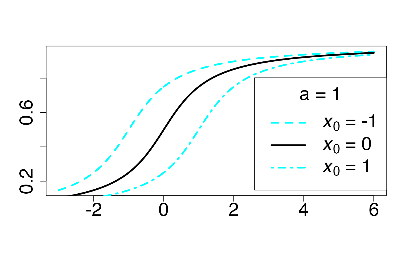
Chemin = "~/Documents/Recherche/DeBoeck/Graphes/Fichiers/"
colmodel="cmyk"
pdf(file = paste(Chemin,"frep_",LOI,".pdf",sep=""),
    width = 8, height = 7, onefile = TRUE, family = "Helvetica",
    title = "Probability or cumulative distribution graphs", paper = "special", colormodel = colmodel)
infx=-3;supx=6;
fr <- function(x) {pcauchy(x,-1)}
curve(fr,from=infx,to=supx,ylab="",xlab="",lty=1,lwd=3,col=colmagentas[1],type="n",cex.axis=2)
curve(fr,from=infx,to=-0.000001,ylab="",xlab="",lty=2,lwd=3,col=colmagentas[2],add=T)
curve(fr,from=0.000001,to=supx,ylab="",xlab="",lty=2,lwd=3,col=colmagentas[2],add=T)
fr <- function(x) {pcauchy(x,0)}
curve(fr,from=infx,to=-0.000001,ylab="",xlab="",lty=1,lwd=3,add=T,col=colmagentas[1])
curve(fr,from=0.000001,to=supx,ylab="",xlab="",lty=1,lwd=3,add=T,col=colmagentas[1])
fr <- function(x) {pcauchy(x,1)}
curve(fr,from=infx,to=-0.000001,ylab="",xlab="",lty=4,lwd=3,add=T,col=colmagentas[3])
curve(fr,from=0.000001,to=supx,ylab="",xlab="",lty=4,lwd=3,add=T,col=colmagentas[3])
leg.txt <- c(expression(paste(italic(x[0])," = -1")), expression(paste(italic(x[0])," = 0")), expression(paste(italic(x[0])," = 1")))
legend("bottomright", leg.txt, title = expression(paste(a," = 1",sep="")), lty = c(2, 1, 4), lwd=3, col = c(colmagentas[2],colmagentas[1],colmagentas[3]), cex = 2, bg="white", inset=c(0,0.0375))# , pch = "*"
dev.off()
#> agg_png 
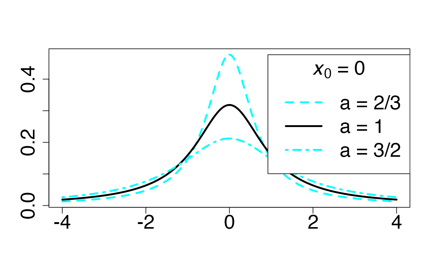
#>       2

Loi de Cauchy (en fonction de $a$)

Fonction de densité de probabilité

Chemin = "~/Documents/Recherche/DeBoeck/Graphes/Fichiers/"
colmodel="cmyk"
pdf(file = paste(Chemin,"dens_",LOI,".pdf",sep=""),
    width = 8, height = 7, onefile = TRUE, family = "Helvetica",
    title = "Probability or cumulative distribution graphs", paper = "special", colormodel = colmodel)
infx=-4;supx=4;
fd <- function(x) {dcauchy(x,0,2/3)}
curve(fd,from=infx,to=supx,ylab="",xlab="",lty=1,lwd=3,col=colmagentas[1],type="n",cex.axis=2)
curve(fd,from=infx,to=-0.000001,ylab="",xlab="",lty=2,lwd=3,add=T,col=colmagentas[2])
curve(fd,from=0.000001,to=supx,ylab="",xlab="",lty=2,lwd=3,add=T,col=colmagentas[2])
fd <- function(x) {dcauchy(x,0,1)}
curve(fd,from=infx,to=-0.000001,ylab="",xlab="",lty=1,lwd=3,add=T,col=colmagentas[1])
curve(fd,from=0.000001,to=supx,ylab="",xlab="",lty=1,lwd=3,add=T,col=colmagentas[1])
fd <- function(x) {dcauchy(x,0,1.5)}
curve(fd,from=infx,to=-0.000001,ylab="",xlab="",lty=4,lwd=3,add=T,col=colmagentas[3])
curve(fd,from=0.000001,to=supx,ylab="",xlab="",lty=4,lwd=3,add=T,col=colmagentas[3])
leg.txt <- c(expression(paste(a," = 2/3",sep="")), expression(paste(a," = 1",sep="")), expression(paste(a," = 3/2",sep="")))
legend("topright", leg.txt, title = expression(paste(italic(x[0])," = 0",sep="")), lty = c(2, 1, 4), lwd=3, col = c(colmagentas[2],colmagentas[1],colmagentas[3]), cex = 2, bg="white", inset=c(0,.0375))# , pch = "*"
dev.off()
#> agg_png 
#>       2

Fonction de répartition

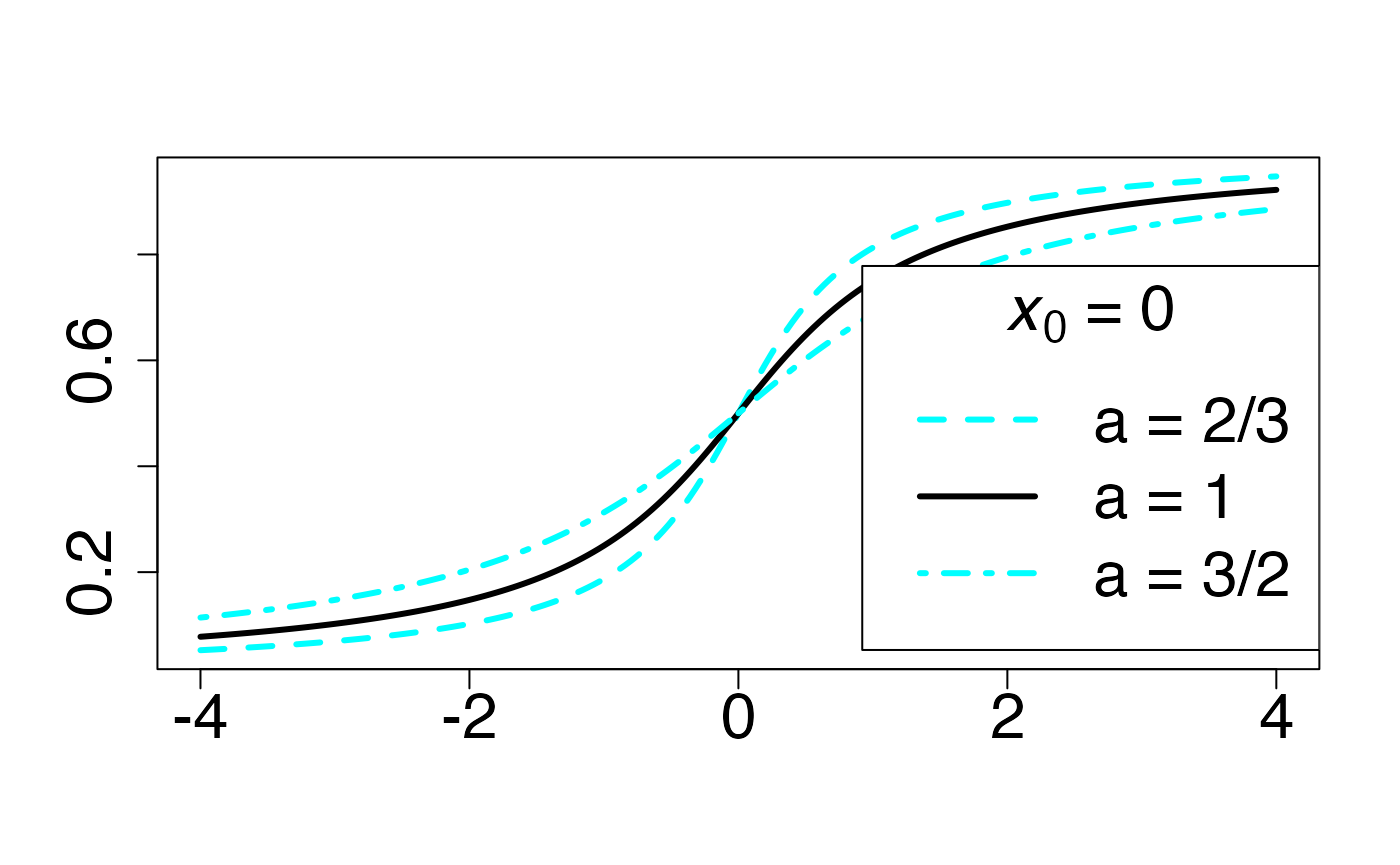
Chemin = "~/Documents/Recherche/DeBoeck/Graphes/Fichiers/"
colmodel="cmyk"
pdf(file = paste(Chemin,"frep_",LOI,".pdf",sep=""),
    width = 8, height = 7, onefile = TRUE, family = "Helvetica",
    title = "Probability or cumulative distribution graphs", paper = "special", colormodel = colmodel)
infx=-4;supx=4;
fd <- function(x) {pcauchy(x,0,2/3)}
curve(fd,from=infx,to=supx,ylab="",xlab="",lty=1,lwd=3,col=colmagentas[1],type="n",cex.axis=2)
curve(fd,from=infx,to=-0.000001,ylab="",xlab="",lty=2,lwd=3,add=T,col=colmagentas[2])
curve(fd,from=0.000001,to=supx,ylab="",xlab="",lty=2,lwd=3,add=T,col=colmagentas[2])
fd <- function(x) {pcauchy(x,0,1)}
curve(fd,from=infx,to=-0.000001,ylab="",xlab="",lty=1,lwd=3,add=T,col=colmagentas[1])
curve(fd,from=0.000001,to=supx,ylab="",xlab="",lty=1,lwd=3,add=T,col=colmagentas[1])
fd <- function(x) {pcauchy(x,0,1.5)}
curve(fd,from=infx,to=-0.000001,ylab="",xlab="",lty=4,lwd=3,add=T,col=colmagentas[3])
curve(fd,from=0.000001,to=supx,ylab="",xlab="",lty=4,lwd=3,add=T,col=colmagentas[3])
leg.txt <- c(expression(paste(a," = 2/3",sep="")), expression(paste(a," = 1",sep="")), expression(paste(a," = 3/2",sep="")))
legend("bottomright", leg.txt, title = expression(paste(italic(x[0])," = 0",sep="")), lty = c(2, 1, 4), lwd=3, col = c(colmagentas[2],colmagentas[1],colmagentas[3]), cex = 2, bg="white", inset=c(0,.0375))# , pch = "*"
dev.off()
#> agg_png 
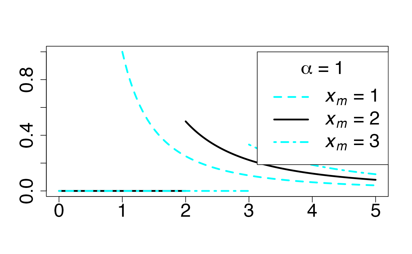
#>       2

Loi de Pareto (en fonction de $x_m$)

Fonction de densité de probabilité

Chemin = "~/Documents/Recherche/DeBoeck/Graphes/Fichiers/"
colmodel="cmyk"
pdf(file = paste(Chemin,"dens_",LOI,".pdf",sep=""),
    width = 8, height = 7, onefile = TRUE, family = "Helvetica",
    title = "Probability or cumulative distribution graphs", paper = "special", colormodel = colmodel)
infx=0;supx=5;
fd <- function(x) {dpareto(x,1,1)}
curve(fd,from=infx,to=supx,ylab="",xlab="",lty=1,lwd=3,col=colmagentas[1],type="n",cex.axis=2)
curve(fd,from=infx,to=1-0.000001,ylab="",xlab="",lty=2,lwd=3,col=colmagentas[2],add=T)
curve(fd,from=1+0.000001,to=supx,ylab="",xlab="",lty=2,lwd=3,col=colmagentas[2],add=T)
fd <- function(x) {dpareto(x,2,1)}
curve(fd,from=infx,to=2-0.000001,ylab="",xlab="",lty=1,lwd=3,add=T,col=colmagentas[1])
curve(fd,from=2+0.000001,to=supx,ylab="",xlab="",lty=1,lwd=3,add=T,col=colmagentas[1])
fd <- function(x) {dpareto(x,3,1)}
curve(fd,from=infx,to=3-0.000001,ylab="",xlab="",lty=4,lwd=3,add=T,col=colmagentas[3])
curve(fd,from=3+0.000001,to=supx,ylab="",xlab="",lty=4,lwd=3,add=T,col=colmagentas[3])
leg.txt <- c(expression(paste(italic(x[m])," = 1")), expression(paste(italic(x[m])," = 2")), expression(paste(italic(x[m])," = 3")))
legend("topright", leg.txt, title = expression(paste(alpha," = 1",sep="")), lty = c(2, 1, 4), lwd=3, col = c(colmagentas[2],colmagentas[1],colmagentas[3]), cex = 2, bg="white", inset=c(0,0.0375))# , pch = "*"
dev.off()
#> agg_png 
#>       2

Fonction de répartition

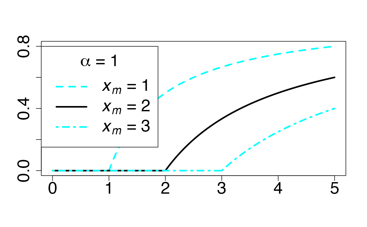
Chemin = "~/Documents/Recherche/DeBoeck/Graphes/Fichiers/"
colmodel="cmyk"
pdf(file = paste(Chemin,"frep_",LOI,".pdf",sep=""),
    width = 8, height = 7, onefile = TRUE, family = "Helvetica",
    title = "Probability or cumulative distribution graphs", paper = "special", colormodel = colmodel)
infx=0;supx=5;
fr <- function(x) {ppareto(x,1,1)}
curve(fr,from=infx,to=supx,ylab="",xlab="",lty=1,lwd=3,col=colmagentas[1],type="n",cex.axis=2)
curve(fr,from=infx,to=1-0.000001,ylab="",xlab="",lty=2,lwd=3,col=colmagentas[2],add=T)
curve(fr,from=1+0.000001,to=supx,ylab="",xlab="",lty=2,lwd=3,col=colmagentas[2],add=T)
fr <- function(x) {ppareto(x,2,1)}
curve(fr,from=infx,to=2-0.000001,ylab="",xlab="",lty=1,lwd=3,add=T,col=colmagentas[1])
curve(fr,from=2+0.000001,to=supx,ylab="",xlab="",lty=1,lwd=3,add=T,col=colmagentas[1])
fr <- function(x) {ppareto(x,3,1)}
curve(fr,from=infx,to=3-0.000001,ylab="",xlab="",lty=4,lwd=3,add=T,col=colmagentas[3])
curve(fr,from=3+0.000001,to=supx,ylab="",xlab="",lty=4,lwd=3,add=T,col=colmagentas[3])
leg.txt <- c(expression(paste(italic(x[m])," = 1")), expression(paste(italic(x[m])," = 2")), expression(paste(italic(x[m])," = 3")))
legend("topleft", leg.txt, title = expression(paste(alpha," = 1",sep="")), lty = c(2, 1, 4), lwd=3, col = c(colmagentas[2],colmagentas[1],colmagentas[3]), cex = 2, bg="white", inset=c(0,0.0375))# , pch = "*"
dev.off()
#> agg_png 
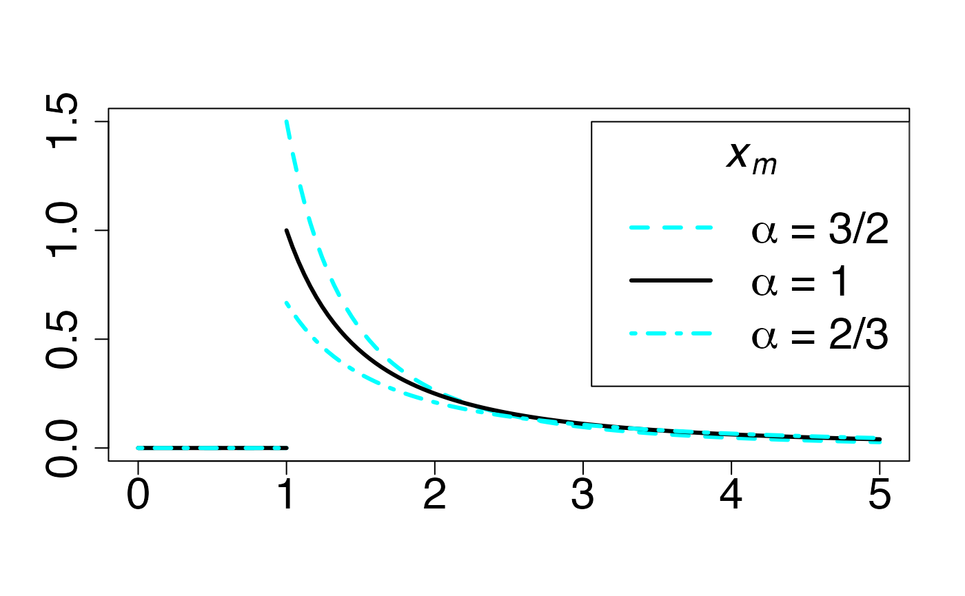
#>       2

Loi de Pareto (en fonction de $\alpha$)

Fonction de densité de probabilité

Chemin = "~/Documents/Recherche/DeBoeck/Graphes/Fichiers/"
colmodel="cmyk"
pdf(file = paste(Chemin,"dens_",LOI,".pdf",sep=""),
    width = 8, height = 7, onefile = TRUE, family = "Helvetica",
    title = "Probability or cumulative distribution graphs", paper = "special", colormodel = colmodel)
infx=0;supx=5;
fd <- function(x) {dpareto(x,1,3/2)}
curve(fd,from=infx,to=supx,ylab="",xlab="",lty=1,lwd=3,col=colmagentas[1],type="n",cex.axis=2)
curve(fd,from=infx,to=1-0.000001,ylab="",xlab="",lty=2,lwd=3,col=colmagentas[2],add=T)
curve(fd,from=1+0.000001,to=supx,ylab="",xlab="",lty=2,lwd=3,col=colmagentas[2],add=T)
fd <- function(x) {dpareto(x,1,1)}
curve(fd,from=infx,to=1-0.000001,ylab="",xlab="",lty=1,lwd=3,add=T,col=colmagentas[1])
curve(fd,from=1+0.000001,to=supx,ylab="",xlab="",lty=1,lwd=3,add=T,col=colmagentas[1])
fd <- function(x) {dpareto(x,1,2/3)}
curve(fd,from=infx,to=1-0.000001,ylab="",xlab="",lty=4,lwd=3,add=T,col=colmagentas[3])
curve(fd,from=1+0.000001,to=supx,ylab="",xlab="",lty=4,lwd=3,add=T,col=colmagentas[3])
leg.txt <- c(expression(paste(italic(alpha)," = 3/2")), expression(paste(italic(alpha)," = 1")), expression(paste(italic(alpha)," = 2/3")))
legend("topright", leg.txt, title = expression(paste(italic(x[m])," = 1",sep="")), lty = c(2, 1, 4), lwd=3, col = c(colmagentas[2],colmagentas[1],colmagentas[3]), cex = 2, bg="white", inset=c(0,0.0375))# , pch = "*"
dev.off()
#> agg_png 
#>       2

Fonction de répartition

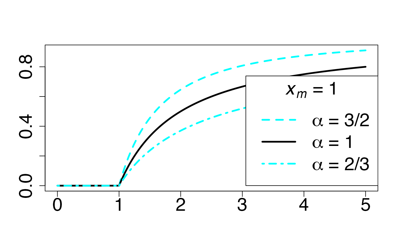
Chemin = "~/Documents/Recherche/DeBoeck/Graphes/Fichiers/"
colmodel="cmyk"
pdf(file = paste(Chemin,"frep_",LOI,".pdf",sep=""),
    width = 8, height = 7, onefile = TRUE, family = "Helvetica",
    title = "Probability or cumulative distribution graphs", paper = "special", colormodel = colmodel)
infx=0;supx=5;
fr <- function(x) {ppareto(x,1,3/2)}
curve(fr,from=infx,to=supx,ylab="",xlab="",lty=1,lwd=3,col=colmagentas[1],type="n",cex.axis=2)
curve(fr,from=infx,to=1-0.000001,ylab="",xlab="",lty=2,lwd=3,col=colmagentas[2],add=T)
curve(fr,from=1+0.000001,to=supx,ylab="",xlab="",lty=2,lwd=3,col=colmagentas[2],add=T)
fr <- function(x) {ppareto(x,1,1)}
curve(fr,from=infx,to=1-0.000001,ylab="",xlab="",lty=1,lwd=3,add=T,col=colmagentas[1])
curve(fr,from=1+0.000001,to=supx,ylab="",xlab="",lty=1,lwd=3,add=T,col=colmagentas[1])
fr <- function(x) {ppareto(x,1,2/3)}
curve(fr,from=infx,to=1-0.000001,ylab="",xlab="",lty=4,lwd=3,add=T,col=colmagentas[3])
curve(fr,from=1+0.000001,to=supx,ylab="",xlab="",lty=4,lwd=3,add=T,col=colmagentas[3])
leg.txt <- c(expression(paste(italic(alpha)," = 3/2")), expression(paste(italic(alpha)," = 1")), expression(paste(italic(alpha)," = 2/3")))
legend("bottomright", leg.txt, title = expression(paste(italic(x[m])," = 1",sep="")), lty = c(2, 1, 4), lwd=3, col = c(colmagentas[2],colmagentas[1],colmagentas[3]), cex = 2, bg="white", inset=c(0,0.0375))# , pch = "*"
dev.off()
#> agg_png 
#>       2