Chapitre 10. Modèles gaussiens de régressions linéaires simple et multiple.

Description des données : Air pollution

Échantillon de 50 villes (individus) tirées aléatoirement sur la pollution de l’air aux États-Unis en 1960

CITY : Nom de la ville
TMR : taux de mortalité exprimé en 1/10000
GE65 : pourcentage (multiplié par 10) de la population des 65 ans et plus
LPOP : logarithme (en base 10 et multiplié par 10) de la population
NONPOOR : pourcentage de ménages avec un revenu au dessus du seuil de pauvreté
PERWH : pourcentage de population blanche * PMEAN : moyenne arithmétique des relevés réalisés deux fois par semaine de particules suspendues dans l’air (micro-g/m3 multiplié par 10)
PMIN : plus petite valeur des relevés réalisés deux fois par semaine de particules suspendues dans l’air (micro-g/m3 multiplié par 10)
LPMAX : logarithme de la plus grande valeur des relevés réalisés deux fois par semaine de particules suspendues dans l’air (micro-g/m3 multiplié par 10)
SMEAN : moyenne arithmétique des relevés réalisés deux fois par semaine de sulfate (micro-g/m3 multiplié par 10)
SMIN : plus petite valeur des relevés réalisés deux fois par semaine de sulfate (micro-g/m3 multiplié par 10)
SMAX : plus grande valeur des relevés réalisés deux fois par semaine de sulfate (micro-g/m3 multiplié par 10)
LPM2 : logarithme de la densité de la population par mile carré (multiplié par 0,1)

Lecture des données

library(sageR)
data(air_pollution)

Élimine les variables PM2 et PMAX qui sont transformées en logarithme dans les variables l_pm2 et l_pmax

air_pollution <- air_pollution[,-(8:9)]

Quelques statistiques descriptives du fichier de données

summary(air_pollution)
#>        CITY         TMR              SMIN            SMEAN       
#>  JACKSON : 2   Min.   : 618.0   Min.   :  1.00   Min.   : 27.00  
#>  AUGUSTA : 1   1st Qu.: 806.5   1st Qu.: 27.25   1st Qu.: 62.25  
#>  AUSTIN  : 1   Median : 882.5   Median : 43.50   Median : 79.50  
#>  BEAUMONT: 1   Mean   : 893.9   Mean   : 47.36   Mean   : 98.18  
#>  BOSTON  : 1   3rd Qu.: 955.2   3rd Qu.: 62.00   3rd Qu.:132.50  
#>  BRIDGEPO: 1   Max.   :1199.0   Max.   :155.00   Max.   :283.00  
#>  (Other) :43                                                     
#>       SMAX            PMIN           PMEAN            PERWH      
#>  Min.   : 58.0   Min.   :10.00   Min.   : 54.00   Min.   :60.00  
#>  1st Qu.:139.5   1st Qu.:29.75   1st Qu.: 90.25   1st Qu.:83.03  
#>  Median :194.5   Median :46.00   Median :121.00   Median :90.65  
#>  Mean   :220.0   Mean   :46.86   Mean   :122.48   Mean   :87.50  
#>  3rd Qu.:265.2   3rd Qu.:57.50   3rd Qu.:147.00   3rd Qu.:95.08  
#>  Max.   :940.0   Max.   :98.00   Max.   :247.00   Max.   :99.30  
#>                                                                  
#>     NONPOOR           GE65             LPOP           l_pm2      
#>  Min.   :67.80   Min.   : 45.00   Min.   :4.937   Min.   :1.808  
#>  1st Qu.:76.58   1st Qu.: 70.25   1st Qu.:5.384   1st Qu.:3.251  
#>  Median :82.65   Median : 81.50   Median :5.570   Median :3.637  
#>  Mean   :81.57   Mean   : 81.32   Mean   :5.639   Mean   :3.814  
#>  3rd Qu.:87.10   3rd Qu.: 93.75   3rd Qu.:5.831   3rd Qu.:4.398  
#>  Max.   :90.70   Max.   :116.00   Max.   :6.794   Max.   :7.213  
#>                                                                  
#>      l_pmax     
#>  Min.   :4.820  
#>  1st Qu.:5.247  
#>  Median :5.489  
#>  Mean   :5.521  
#>  3rd Qu.:5.777  
#>  Max.   :6.865  
#>

Exercice 10.1 : Analyse des corrélations entre les variables

GGally::ggpairs(air_pollution[,-1], progress = FALSE)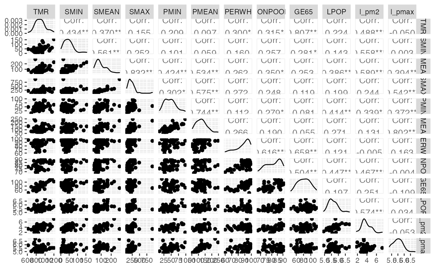
#> Registered S3 method overwritten by 'GGally':
#>   method from   
#>   +.gg   ggplot2

cor_pollution <- cor(air_pollution[,-1])
col1 <- colorRampPalette(c("#7F0000", "red", "#FF7F00", "yellow", "white",
                           "cyan", "#007FFF", "blue", "#00007F"))
col2 <- colorRampPalette(c("#67001F", "#B2182B", "#D6604D", "#F4A582",
                           "#FDDBC7", "#FFFFFF", "#D1E5F0", "#92C5DE",
                           "#4393C3", "#2166AC", "#053061"))
col3 <- colorRampPalette(c("red", "white", "blue")) 
col4 <- colorRampPalette(c("#7F0000", "red", "#FF7F00", "yellow", "#7FFF7F",
                           "cyan", "#007FFF", "blue", "#00007F"))
whiteblack <- c("white", "black")
corrplot::corrplot(cor_pollution, method = "color", addrect = 2, col = col1(100))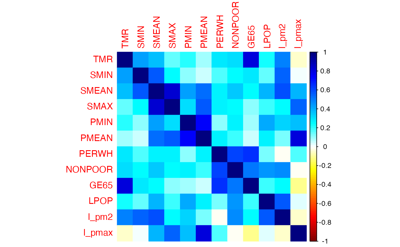

Exercice 10.2 : Régression simple

reg_TMR_GE65 <- lm(TMR~GE65,data=air_pollution)
summary(reg_TMR_GE65)
#> 
#> Call:
#> lm(formula = TMR ~ GE65, data = air_pollution)
#> 
#> Residuals:
#>      Min       1Q   Median       3Q      Max 
#> -174.287  -39.126   -8.287   49.514  189.929 
#> 
#> Coefficients:
#>             Estimate Std. Error t value Pr(>|t|)    
#> (Intercept) 426.5237    50.4206   8.459 4.49e-11 ***
#> GE65          5.7469     0.6073   9.464 1.49e-12 ***
#> ---
#> Signif. codes:  0 '***' 0.001 '**' 0.01 '*' 0.05 '.' 0.1 ' ' 1
#> 
#> Residual standard error: 71.97 on 48 degrees of freedom
#> Multiple R-squared:  0.6511, Adjusted R-squared:  0.6438 
#> F-statistic: 89.56 on 1 and 48 DF,  p-value: 1.492e-12

reg_TMR_LPOP <- lm(TMR~LPOP,data=air_pollution)
summary(reg_TMR_LPOP)
#> 
#> Call:
#> lm(formula = TMR ~ LPOP, data = air_pollution)
#> 
#> Residuals:
#>      Min       1Q   Median       3Q      Max 
#> -265.725  -73.857   -0.878   60.211  294.585 
#> 
#> Coefficients:
#>             Estimate Std. Error t value Pr(>|t|)  
#> (Intercept)   489.92     254.18   1.927   0.0599 .
#> LPOP           71.64      44.98   1.593   0.1178  
#> ---
#> Signif. codes:  0 '***' 0.001 '**' 0.01 '*' 0.05 '.' 0.1 ' ' 1
#> 
#> Residual standard error: 118.7 on 48 degrees of freedom
#> Multiple R-squared:  0.05019,    Adjusted R-squared:  0.0304 
#> F-statistic: 2.537 on 1 and 48 DF,  p-value: 0.1178

reg_TMR_NONPOOR <- lm(TMR~NONPOOR,data=air_pollution)
summary(reg_TMR_NONPOOR)
#> 
#> Call:
#> lm(formula = TMR ~ NONPOOR, data = air_pollution)
#> 
#> Residuals:
#>      Min       1Q   Median       3Q      Max 
#> -253.912  -84.067   -7.787   43.187  270.812 
#> 
#> Coefficients:
#>             Estimate Std. Error t value Pr(>|t|)  
#> (Intercept)  405.541    212.736   1.906   0.0626 .
#> NONPOOR        5.987      2.600   2.302   0.0257 *
#> ---
#> Signif. codes:  0 '***' 0.001 '**' 0.01 '*' 0.05 '.' 0.1 ' ' 1
#> 
#> Residual standard error: 115.6 on 48 degrees of freedom
#> Multiple R-squared:  0.09944,    Adjusted R-squared:  0.08068 
#> F-statistic:   5.3 on 1 and 48 DF,  p-value: 0.0257

reg_TMR_PERWH <- lm(TMR~PERWH,data=air_pollution)
summary(reg_TMR_PERWH)
#> 
#> Call:
#> lm(formula = TMR ~ PERWH, data = air_pollution)
#> 
#> Residuals:
#>      Min       1Q   Median       3Q      Max 
#> -307.890  -67.430    4.312   58.856  285.641 
#> 
#> Coefficients:
#>             Estimate Std. Error t value Pr(>|t|)    
#> (Intercept)  589.299    141.000   4.179 0.000123 ***
#> PERWH          3.481      1.600   2.175 0.034602 *  
#> ---
#> Signif. codes:  0 '***' 0.001 '**' 0.01 '*' 0.05 '.' 0.1 ' ' 1
#> 
#> Residual standard error: 116.2 on 48 degrees of freedom
#> Multiple R-squared:  0.0897, Adjusted R-squared:  0.07074 
#> F-statistic:  4.73 on 1 and 48 DF,  p-value: 0.0346

reg_TMR_PMEAN <- lm(TMR~PMEAN,data=air_pollution)
summary(reg_TMR_PMEAN)
#> 
#> Call:
#> lm(formula = TMR ~ PMEAN, data = air_pollution)
#> 
#> Residuals:
#>      Min       1Q   Median       3Q      Max 
#> -283.601  -82.968    0.699   58.449  298.242 
#> 
#> Coefficients:
#>             Estimate Std. Error t value Pr(>|t|)    
#> (Intercept) 859.4062    53.7979  15.975   <2e-16 ***
#> PMEAN         0.2813     0.4163   0.676    0.502    
#> ---
#> Signif. codes:  0 '***' 0.001 '**' 0.01 '*' 0.05 '.' 0.1 ' ' 1
#> 
#> Residual standard error: 121.3 on 48 degrees of freedom
#> Multiple R-squared:  0.009422,   Adjusted R-squared:  -0.01122 
#> F-statistic: 0.4565 on 1 and 48 DF,  p-value: 0.5025

reg_TMR_PMIN <- lm(TMR~PMIN,data=air_pollution)
summary(reg_TMR_PMIN)
#> 
#> Call:
#> lm(formula = TMR ~ PMIN, data = air_pollution)
#> 
#> Residuals:
#>      Min       1Q   Median       3Q      Max 
#> -278.532  -77.940    6.705   52.070  299.172 
#> 
#> Coefficients:
#>             Estimate Std. Error t value Pr(>|t|)    
#> (Intercept) 835.3543    42.9612   19.44   <2e-16 ***
#> PMIN          1.2485     0.8433    1.48    0.145    
#> ---
#> Signif. codes:  0 '***' 0.001 '**' 0.01 '*' 0.05 '.' 0.1 ' ' 1
#> 
#> Residual standard error: 119.1 on 48 degrees of freedom
#> Multiple R-squared:  0.04367,    Adjusted R-squared:  0.02374 
#> F-statistic: 2.192 on 1 and 48 DF,  p-value: 0.1453

reg_TMR_l_pmax <- lm(TMR~l_pmax,data=air_pollution)
summary(reg_TMR_l_pmax)
#> 
#> Call:
#> lm(formula = TMR ~ l_pmax, data = air_pollution)
#> 
#> Residuals:
#>     Min      1Q  Median      3Q     Max 
#> -270.50  -86.47  -10.79   67.23  305.31 
#> 
#> Coefficients:
#>             Estimate Std. Error t value Pr(>|t|)    
#> (Intercept)   967.71     212.38   4.556 3.58e-05 ***
#> l_pmax        -13.38      38.34  -0.349    0.729    
#> ---
#> Signif. codes:  0 '***' 0.001 '**' 0.01 '*' 0.05 '.' 0.1 ' ' 1
#> 
#> Residual standard error: 121.7 on 48 degrees of freedom
#> Multiple R-squared:  0.002529,   Adjusted R-squared:  -0.01825 
#> F-statistic: 0.1217 on 1 and 48 DF,  p-value: 0.7287

reg_TMR_SMEAN <- lm(TMR~SMEAN,data=air_pollution)
summary(reg_TMR_SMEAN)
#> 
#> Call:
#> lm(formula = TMR ~ SMEAN, data = air_pollution)
#> 
#> Residuals:
#>      Min       1Q   Median       3Q      Max 
#> -266.672  -62.242   -0.821   57.914  278.902 
#> 
#> Coefficients:
#>             Estimate Std. Error t value Pr(>|t|)    
#> (Intercept) 813.1775    33.3272   24.40  < 2e-16 ***
#> SMEAN         0.8218     0.2977    2.76  0.00816 ** 
#> ---
#> Signif. codes:  0 '***' 0.001 '**' 0.01 '*' 0.05 '.' 0.1 ' ' 1
#> 
#> Residual standard error: 113.2 on 48 degrees of freedom
#> Multiple R-squared:  0.137,  Adjusted R-squared:  0.119 
#> F-statistic: 7.618 on 1 and 48 DF,  p-value: 0.008158

reg_TMR_SMIN <- lm(TMR~SMIN,data=air_pollution)
summary(reg_TMR_SMIN)
#> 
#> Call:
#> lm(formula = TMR ~ SMIN, data = air_pollution)
#> 
#> Residuals:
#>      Min       1Q   Median       3Q      Max 
#> -275.271  -73.666   -1.265   68.334  239.169 
#> 
#> Coefficients:
#>             Estimate Std. Error t value Pr(>|t|)    
#> (Intercept) 816.3143    27.9532  29.203  < 2e-16 ***
#> SMIN          1.6374     0.4908   3.336  0.00165 ** 
#> ---
#> Signif. codes:  0 '***' 0.001 '**' 0.01 '*' 0.05 '.' 0.1 ' ' 1
#> 
#> Residual standard error: 109.8 on 48 degrees of freedom
#> Multiple R-squared:  0.1882, Adjusted R-squared:  0.1713 
#> F-statistic: 11.13 on 1 and 48 DF,  p-value: 0.001647

reg_TMR_SMAX <- lm(TMR~SMAX,data=air_pollution)
summary(reg_TMR_SMAX)
#> 
#> Call:
#> lm(formula = TMR ~ SMAX, data = air_pollution)
#> 
#> Residuals:
#>      Min       1Q   Median       3Q      Max 
#> -274.103  -81.565   -1.544   57.872  288.864 
#> 
#> Coefficients:
#>             Estimate Std. Error t value Pr(>|t|)    
#> (Intercept) 864.0365    32.3440  26.714   <2e-16 ***
#> SMAX          0.1356     0.1250   1.084    0.284    
#> ---
#> Signif. codes:  0 '***' 0.001 '**' 0.01 '*' 0.05 '.' 0.1 ' ' 1
#> 
#> Residual standard error: 120.4 on 48 degrees of freedom
#> Multiple R-squared:  0.02391,    Adjusted R-squared:  0.003578 
#> F-statistic: 1.176 on 1 and 48 DF,  p-value: 0.2836

reg_TMR_l_pm2 <- lm(TMR~l_pm2,data=air_pollution)
summary(reg_TMR_l_pm2)
#> 
#> Call:
#> lm(formula = TMR ~ l_pm2, data = air_pollution)
#> 
#> Residuals:
#>      Min       1Q   Median       3Q      Max 
#> -250.718  -59.062   -5.373   72.194  241.352 
#> 
#> Coefficients:
#>             Estimate Std. Error t value Pr(>|t|)    
#> (Intercept)   665.05      60.97  10.908 1.36e-14 ***
#> l_pm2          60.00      15.49   3.873 0.000325 ***
#> ---
#> Signif. codes:  0 '***' 0.001 '**' 0.01 '*' 0.05 '.' 0.1 ' ' 1
#> 
#> Residual standard error: 106.3 on 48 degrees of freedom
#> Multiple R-squared:  0.2381, Adjusted R-squared:  0.2222 
#> F-statistic:    15 on 1 and 48 DF,  p-value: 0.0003254

Exercice 10.3 : Analyse des résidus et des observations

Analyse du modèle TMR vs GE65

par(oma=c(0,12,1,5)+1,bg="white")
plot(air_pollution$GE65, air_pollution$TMR, type = "n",xlab="GE65",ylab="TMR",main="Evolution de TMR en fonction de GE65")
text(air_pollution$GE65, air_pollution$TMR, air_pollution$CITY,col='black',cex=0.7)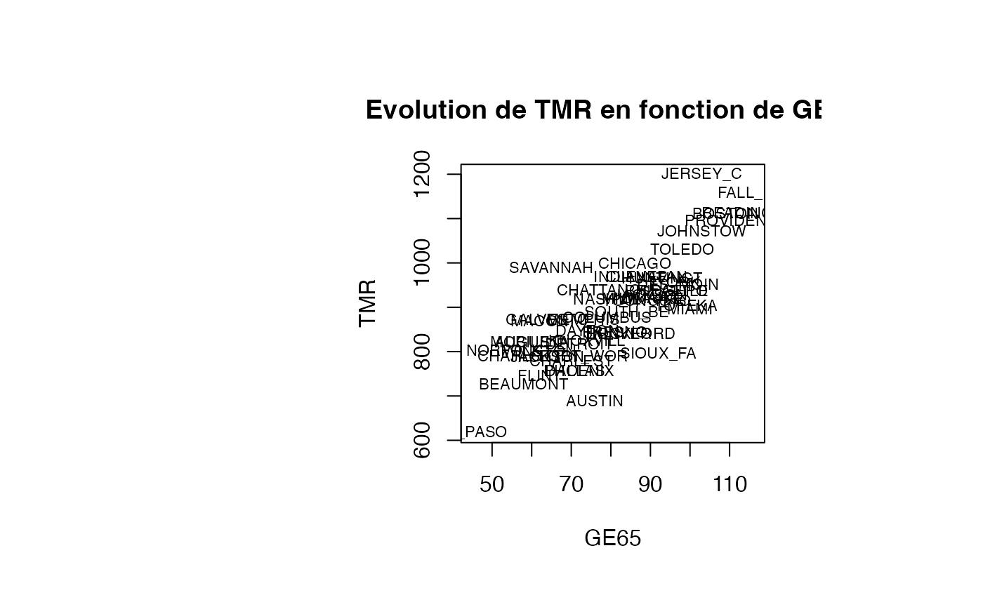

rstudent_leverage <- olsrr::ols_prep_rstudlev_data(reg_TMR_GE65)
rstudent <- rstudent_leverage$levrstud$rstudent
result_TMR_GE65 <- data.frame(air_pollution,rstudent)
par(oma=c(0,12,1,5)+1,bg="white")
plot(result_TMR_GE65$GE65, result_TMR_GE65$rstudent, type = "n",xlab="GE65",ylab="RStudents",main="Comportement des RStudents")
text(result_TMR_GE65$GE65, result_TMR_GE65$rstudent, result_TMR_GE65$CITY,col='black',cex=0.7)
abline(h=c(-1.99,0,1.99))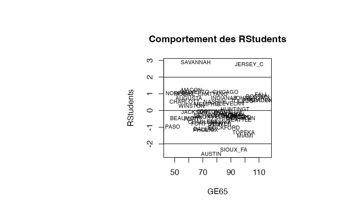

leverage <- rstudent_leverage$levrstud$leverage
result_TMR_GE65 <- data.frame(result_TMR_GE65,leverage)
par(oma=c(0,12,1,5)+1,bg="white")
plot(result_TMR_GE65$GE65, result_TMR_GE65$leverage, type = "n",xlab="GE65",ylab="Levier",main="Comportement des leviers")
text(result_TMR_GE65$GE65, result_TMR_GE65$leverage, result_TMR_GE65$CITY,col='black',cex=0.7)
abline(h=0.08)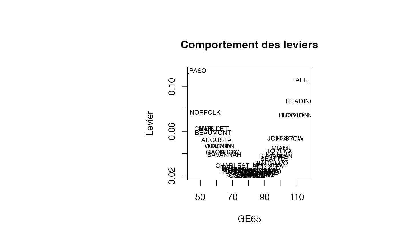

resid <- reg_TMR_GE65$residuals
rmse <- sqrt(49*var(resid)/48)
resid_std <- resid/rmse

cookd <- matrix(0,nrow=50)
for (i in 1:50)
    {cookd[i]=(leverage[i]/(1-leverage[i]))*(resid_std[i]^2/(2*(1-leverage[i])))}
result_TMR_GE65 <- data.frame(result_TMR_GE65,cookd)
par(oma=c(0,12,1,5)+1,bg="white")
plot(result_TMR_GE65$GE65, result_TMR_GE65$cookd, type = "n",xlab="GE65",ylab="D de Cook",main="Comportement des D de Cook")
text(result_TMR_GE65$GE65, result_TMR_GE65$cookd, result_TMR_GE65$CITY,col='black',cex=0.7)
abline(h=0.08)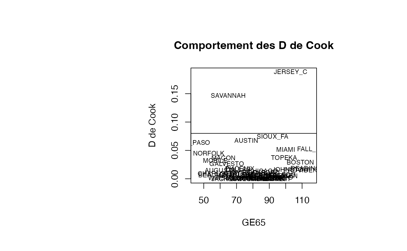

Analyse du modèle TMR vs l_pm2

par(oma=c(0,12,1,5)+1,bg="white")
plot(air_pollution$l_pm2, air_pollution$TMR, type = "n",xlab="l_pm2",ylab="TMR",main="Evolution de TMR en fonction de l_pm2")
text(air_pollution$l_pm2, air_pollution$TMR, air_pollution$CITY,col='black',cex=0.7)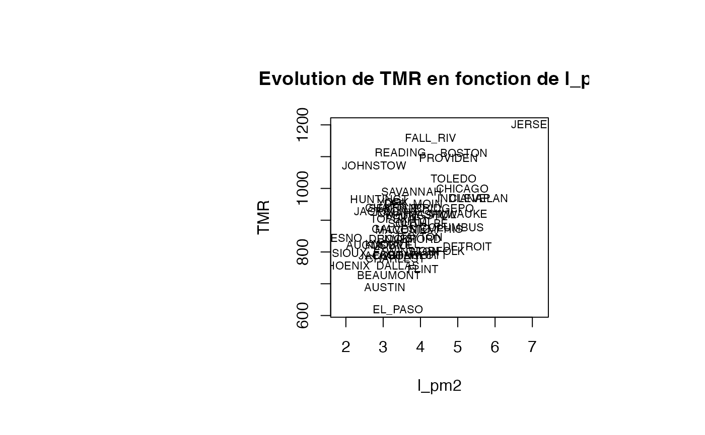

rstudent_leverage <- olsrr::ols_prep_rstudlev_data(reg_TMR_l_pm2)
rstudent <- rstudent_leverage$levrstud$rstudent
result_TMR_l_pm2 <- data.frame(air_pollution,rstudent)
par(oma=c(0,12,1,5)+1,bg="white")
plot(result_TMR_l_pm2$l_pm2, result_TMR_l_pm2$rstudent, type = "n",xlab="l_pm2",ylab="RStudents",main="Comportement des RStudents")
text(result_TMR_l_pm2$l_pm2, result_TMR_l_pm2$rstudent, result_TMR_l_pm2$CITY,col='black',cex=0.7)
abline(h=c(-1.99,0,1.99))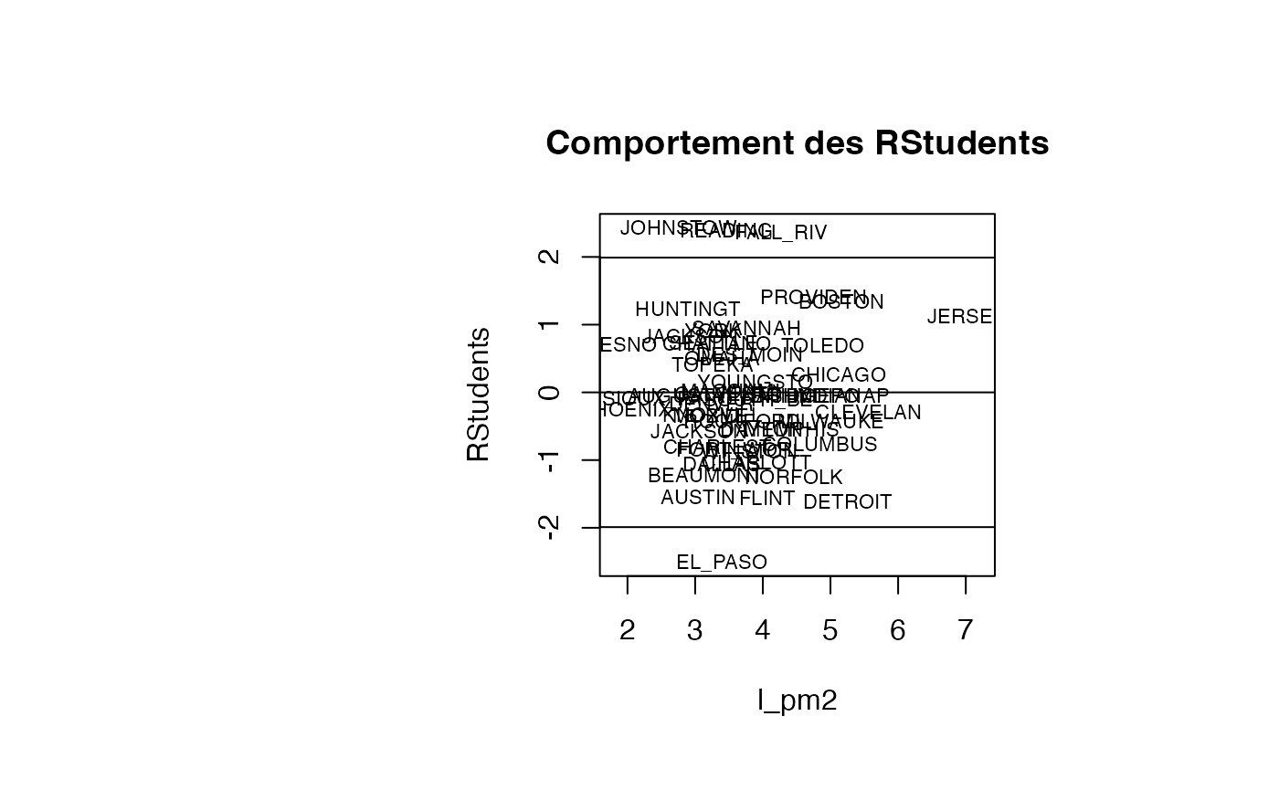

leverage <- rstudent_leverage$levrstud$leverage
result_TMR_l_pm2 <- data.frame(result_TMR_l_pm2,leverage)
par(oma=c(0,12,1,5)+1,bg="white")
plot(result_TMR_l_pm2$l_pm2, result_TMR_l_pm2$leverage, type = "n",xlab="l_pm2",ylab="Levier",main="Comportement des leviers")
text(result_TMR_l_pm2$l_pm2, result_TMR_l_pm2$leverage, result_TMR_l_pm2$CITY,col='black',cex=0.7)
abline(h=0.08)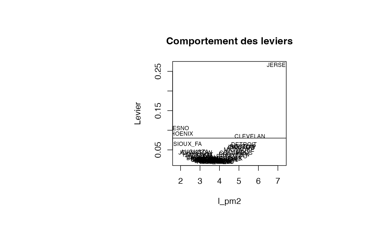

resid <- reg_TMR_l_pm2$residuals
rmse <- sqrt(49*var(resid)/48)
resid_std <- resid/rmse

cookd <- matrix(0,nrow=50)
for (i in 1:50)
    {cookd[i]=(leverage[i]/(1-leverage[i]))*(resid_std[i]^2/(2*(1-leverage[i])))}
result_TMR_l_pm2 <- data.frame(result_TMR_l_pm2,cookd)
par(oma=c(0,12,1,5)+1,bg="white")
plot(result_TMR_l_pm2$l_pm2, result_TMR_l_pm2$cookd, type = "n",xlab="l_pm2",ylab="D de Cook",main="Comportement des D de Cook")
text(result_TMR_l_pm2$l_pm2, result_TMR_l_pm2$cookd, result_TMR_l_pm2$CITY,col='black',cex=0.7)
abline(h=0.08)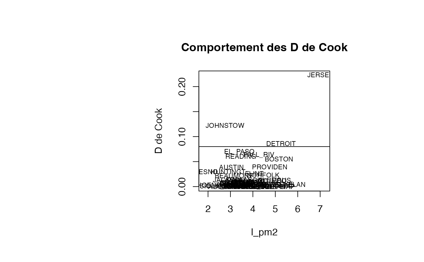

Analyse du modèle TMR vs SMIN

par(oma=c(0,12,1,5)+1,bg="white")
plot(air_pollution$SMIN, air_pollution$TMR, type = "n",xlab="SMIN",ylab="TMR",main="Evolution de TMR en fonction de SMIN")
text(air_pollution$SMIN, air_pollution$TMR, air_pollution$CITY,col='black',cex=0.7)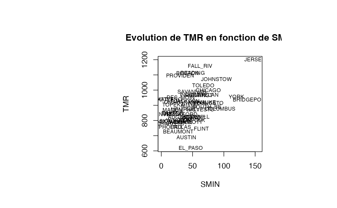

rstudent_leverage <- olsrr::ols_prep_rstudlev_data(reg_TMR_SMIN)
rstudent <- rstudent_leverage$levrstud$rstudent
result_TMR_SMIN <- data.frame(air_pollution,rstudent)
par(oma=c(0,12,1,5)+1,bg="white")
plot(result_TMR_SMIN$SMIN, result_TMR_SMIN$rstudent, type = "n",xlab="SMIN",ylab="RStudents",main="Comportement des RStudents")
text(result_TMR_SMIN$SMIN, result_TMR_SMIN$rstudent, result_TMR_SMIN$CITY,col='black',cex=0.7)
abline(h=c(-1.99,0,1.99))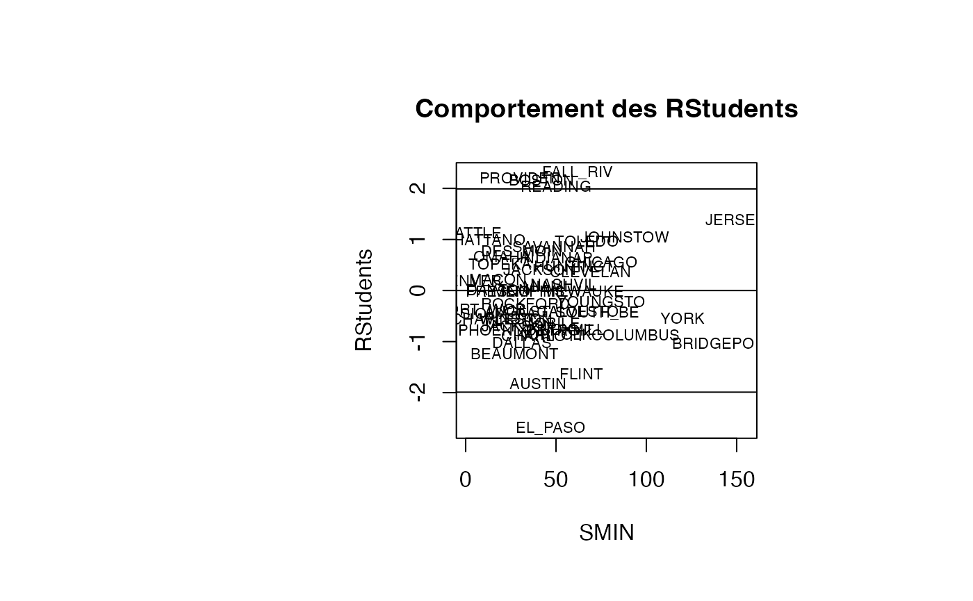

leverage <- rstudent_leverage$levrstud$leverage
result_TMR_SMIN <- data.frame(result_TMR_SMIN,leverage)
par(oma=c(0,12,1,5)+1,bg="white")
plot(result_TMR_SMIN$SMIN, result_TMR_SMIN$leverage, type = "n",xlab="SMIN",ylab="Levier",main="Comportement des leviers")
text(result_TMR_SMIN$SMIN, result_TMR_SMIN$leverage, result_TMR_SMIN$CITY,col='black',cex=0.7)
abline(h=0.08)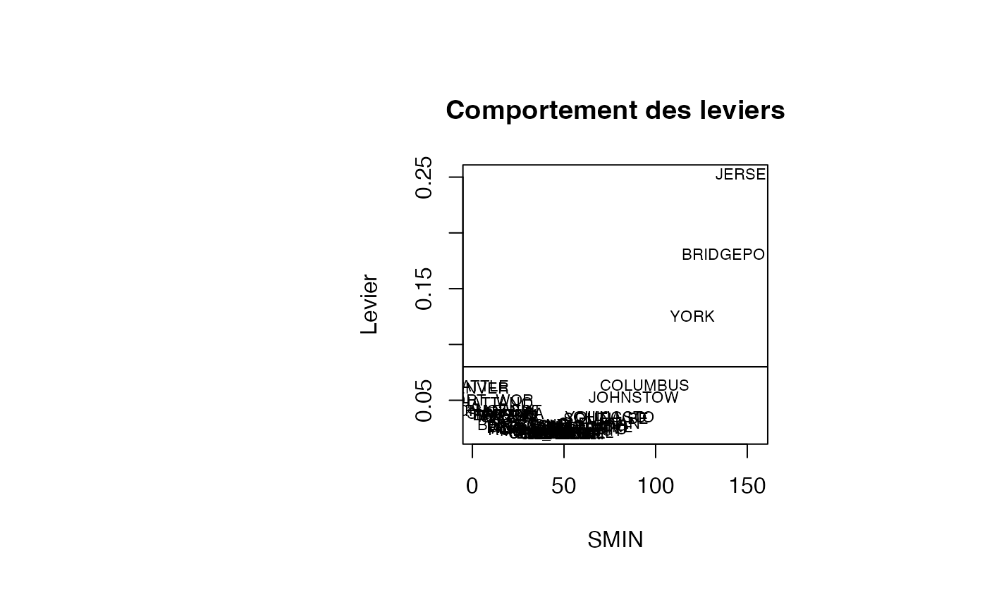

resid <- reg_TMR_SMIN$residuals
rmse <- sqrt(49*var(resid)/48)
resid_std <- resid/rmse

cookd <- matrix(0,nrow=50)
for (i in 1:50)
    {cookd[i]=(leverage[i]/(1-leverage[i]))*(resid_std[i]^2/(2*(1-leverage[i])))}
result_TMR_SMIN <- data.frame(result_TMR_SMIN,cookd)
par(oma=c(0,12,1,5)+1,bg="white")
plot(result_TMR_SMIN$SMIN, result_TMR_SMIN$cookd, type = "n",xlab="SMIN",ylab="D de Cook",main="Comportement des D de Cook")
text(result_TMR_SMIN$SMIN, result_TMR_SMIN$cookd, result_TMR_SMIN$CITY,col='black',cex=0.7)
abline(h=0.08)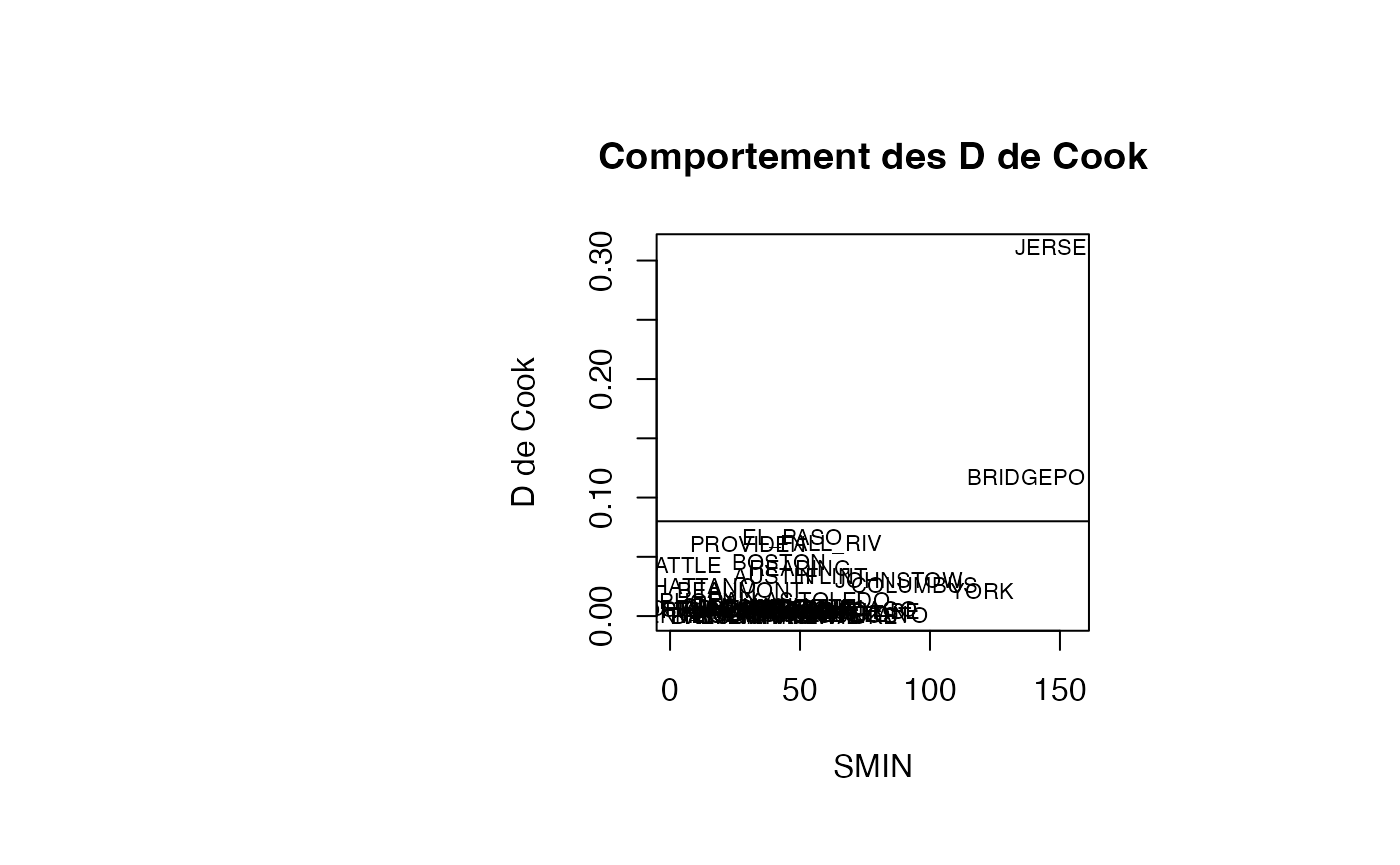

Analyse du modèle TMR vs SMEAN

par(oma=c(0,12,1,5)+1,bg="white")
plot(air_pollution$SMEAN, air_pollution$TMR, type = "n",xlab="SMEAN",ylab="TMR",main="Evolution de TMR en fonction de SMEAN")
text(air_pollution$SMEAN, air_pollution$TMR, air_pollution$CITY,col='black',cex=0.7)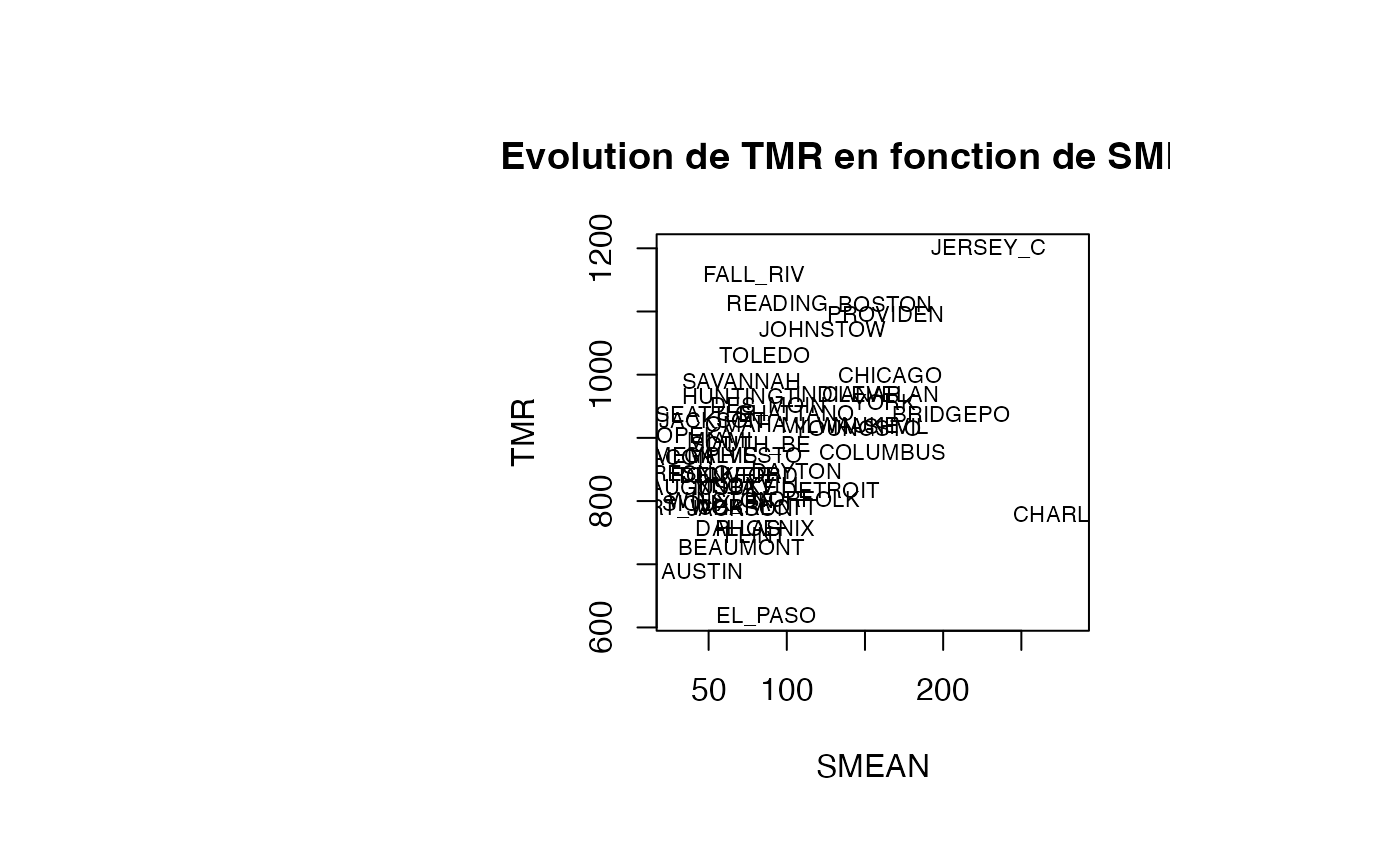

rstudent_leverage <- olsrr::ols_prep_rstudlev_data(reg_TMR_SMEAN)
rstudent <- rstudent_leverage$levrstud$rstudent
result_TMR_SMEAN <- data.frame(air_pollution,rstudent)
par(oma=c(0,12,1,5)+1,bg="white")
plot(result_TMR_SMEAN$SMEAN, result_TMR_SMEAN$rstudent, type = "n",xlab="SMEAN",ylab="RStudents",main="Comportement des RStudents")
text(result_TMR_SMEAN$SMEAN, result_TMR_SMEAN$rstudent, result_TMR_SMEAN$CITY,col='black',cex=0.7)
abline(h=c(-1.99,0,1.99))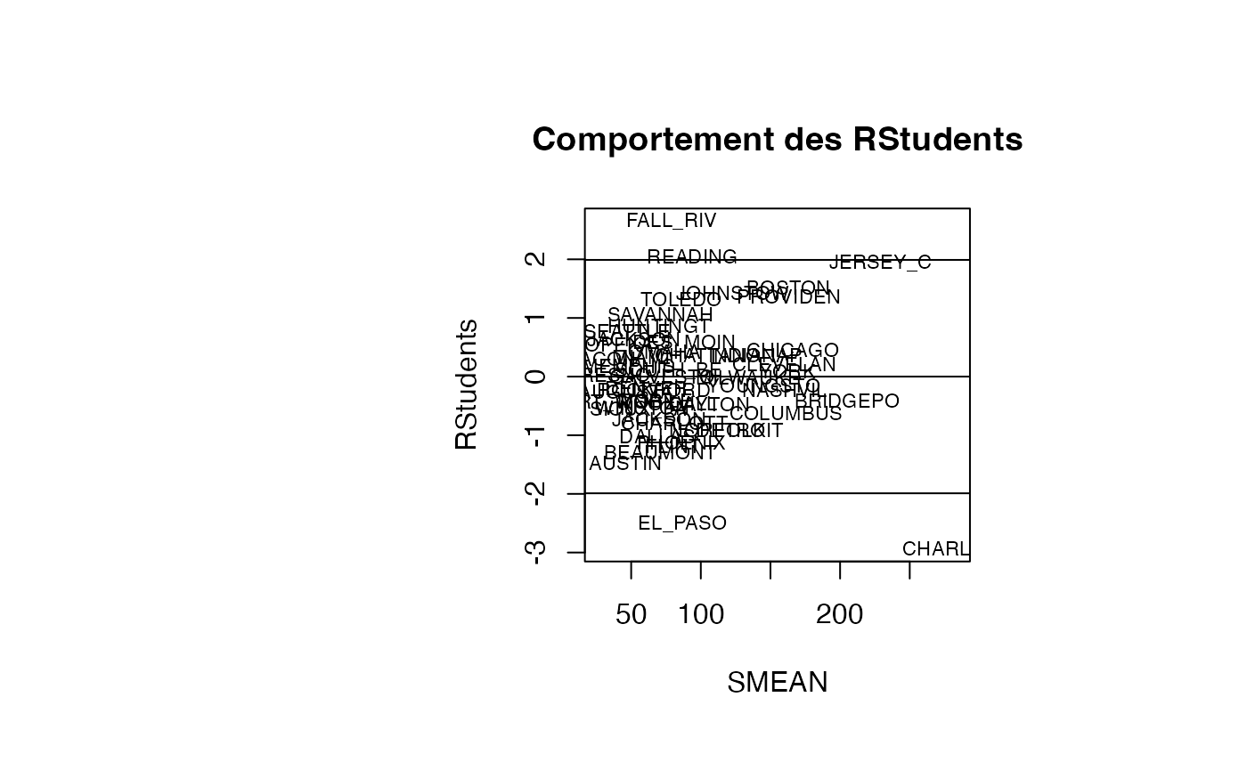

leverage <- rstudent_leverage$levrstud$leverage
result_TMR_SMEAN <- data.frame(result_TMR_SMEAN,leverage)
par(oma=c(0,12,1,5)+1,bg="white")
plot(result_TMR_SMEAN$SMEAN, result_TMR_SMEAN$leverage, type = "n",xlab="SMEAN",ylab="Levier",main="Comportement des leviers")
text(result_TMR_SMEAN$SMEAN, result_TMR_SMEAN$leverage, result_TMR_SMEAN$CITY,col='black',cex=0.7)
abline(h=0.08)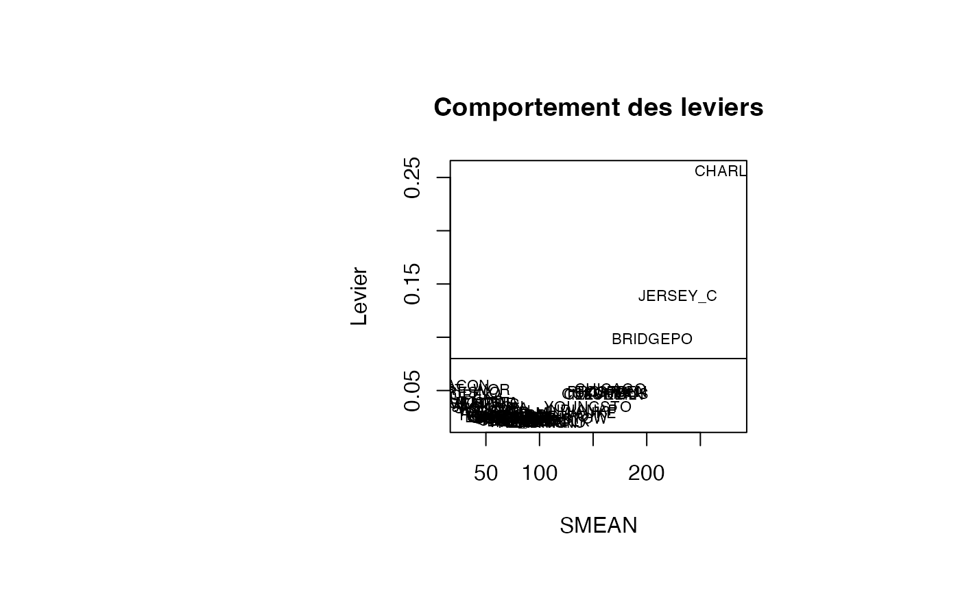

resid <- reg_TMR_SMEAN$residuals
rmse <- sqrt(49*var(resid)/48)
resid_std <- resid/rmse

cookd <- matrix(0,nrow=50)
for (i in 1:50)
    {cookd[i]=(leverage[i]/(1-leverage[i]))*(resid_std[i]^2/(2*(1-leverage[i])))}
result_TMR_SMEAN <- data.frame(result_TMR_SMEAN,cookd)
par(oma=c(0,12,1,5)+1,bg="white")
plot(result_TMR_SMEAN$SMEAN, result_TMR_SMEAN$cookd, type = "n",xlab="SMEAN",ylab="D de Cook",main="Comportement des D de Cook")
text(result_TMR_SMEAN$SMEAN, result_TMR_SMEAN$cookd, result_TMR_SMEAN$CITY,col='black',cex=0.7)
abline(h=0.08)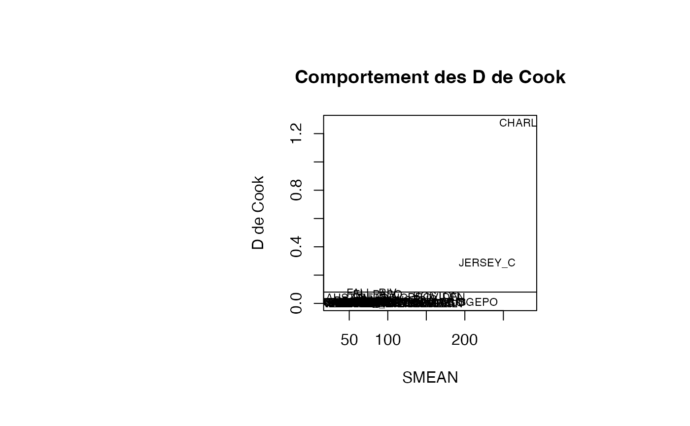

Analyse du modèle TMR vs NOOPOOR

par(oma=c(0,12,1,5)+1,bg="white")
plot(air_pollution$NONPOOR, air_pollution$TMR, type = "n",xlab="NONPOOR",ylab="TMR",main="Evolution de TMR en fonction de NONPOOR")
text(air_pollution$NONPOOR, air_pollution$TMR, air_pollution$CITY,col='black',cex=0.7)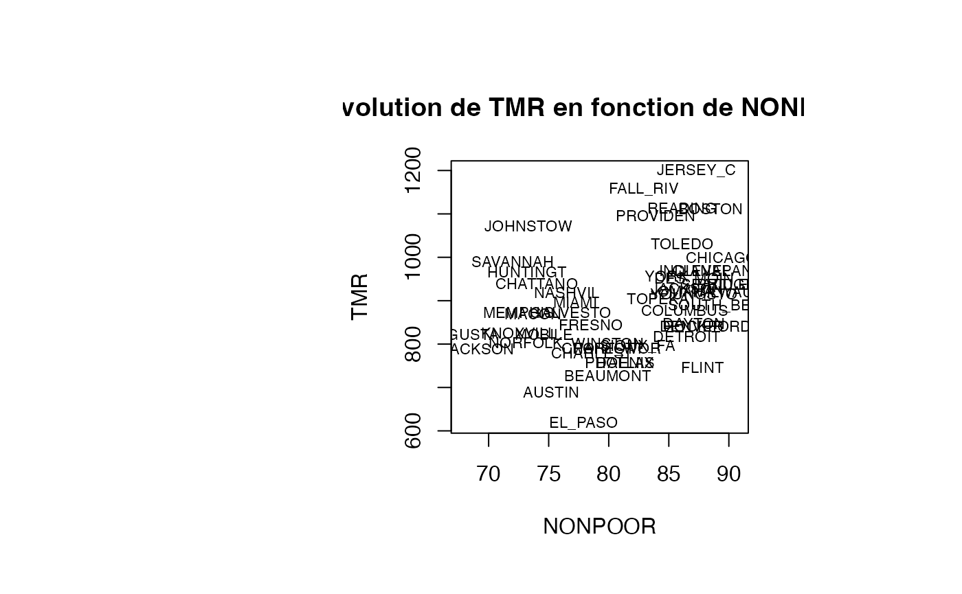

rstudent_leverage <- olsrr::ols_prep_rstudlev_data(reg_TMR_NONPOOR)
rstudent <- rstudent_leverage$levrstud$rstudent
result_TMR_NONPOOR <- data.frame(air_pollution,rstudent)
par(oma=c(0,12,1,5)+1,bg="white")
plot(result_TMR_NONPOOR$NONPOOR, result_TMR_NONPOOR$rstudent, type = "n",xlab="NONPOOR",ylab="RStudents",main="Comportement des RStudents")
text(result_TMR_NONPOOR$NONPOOR, result_TMR_NONPOOR$rstudent, result_TMR_NONPOOR$CITY,col='black',cex=0.7)
abline(h=c(-1.99,0,1.99))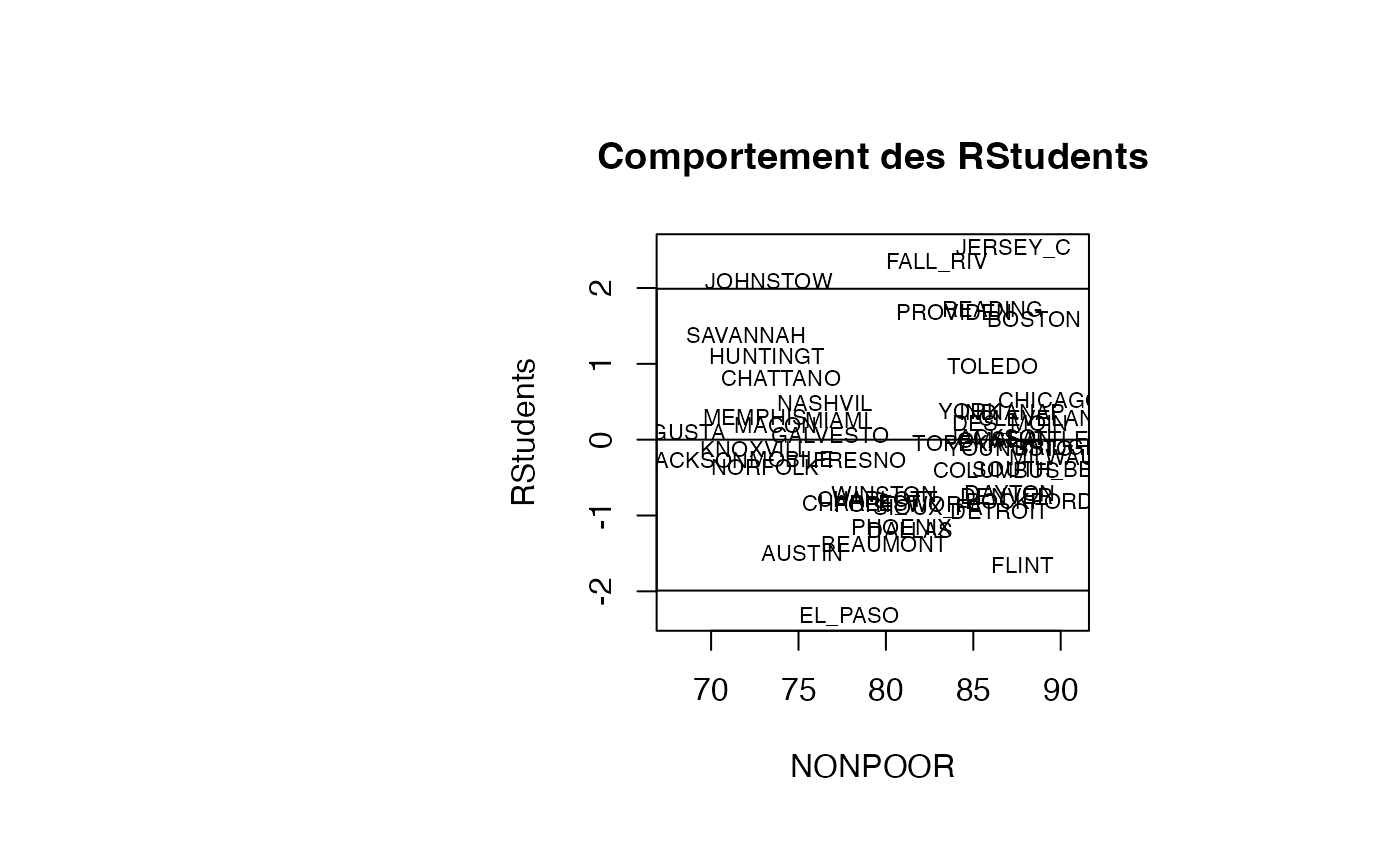

leverage <- rstudent_leverage$levrstud$leverage
result_TMR_NONPOOR <- data.frame(result_TMR_NONPOOR,leverage)
par(oma=c(0,12,1,5)+1,bg="white")
plot(result_TMR_NONPOOR$NONPOOR, result_TMR_NONPOOR$leverage, type = "n",xlab="NONPOOR",ylab="Levier",main="Comportement des leviers")
text(result_TMR_NONPOOR$NONPOOR, result_TMR_NONPOOR$leverage, result_TMR_NONPOOR$CITY,col='black',cex=0.7)
abline(h=0.08)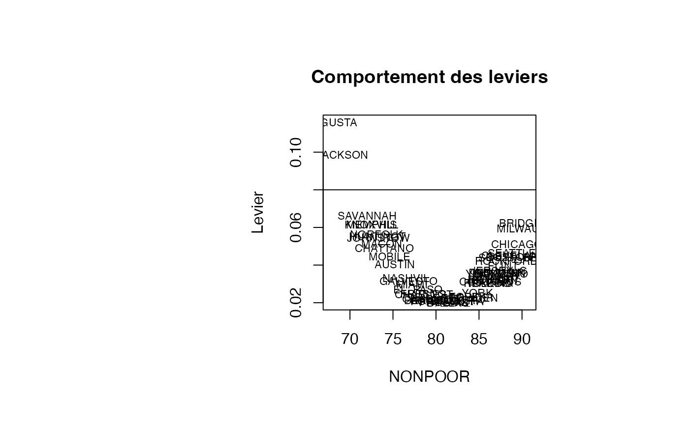

resid <- reg_TMR_NONPOOR$residuals
rmse <- sqrt(49*var(resid)/48)
resid_std <- resid/rmse

cookd <- matrix(0,nrow=50)
for (i in 1:50)
    {cookd[i]=(leverage[i]/(1-leverage[i]))*(resid_std[i]^2/(2*(1-leverage[i])))}
result_TMR_NONPOOR <- data.frame(result_TMR_NONPOOR,cookd)
par(oma=c(0,12,1,5)+1,bg="white")
plot(result_TMR_NONPOOR$NONPOOR, result_TMR_NONPOOR$cookd, type = "n",xlab="NONPOOR",ylab="D de Cook",main="Comportement des D de Cook")
text(result_TMR_NONPOOR$NONPOOR, result_TMR_NONPOOR$cookd, result_TMR_NONPOOR$CITY,col='black',cex=0.7)
abline(h=0.08)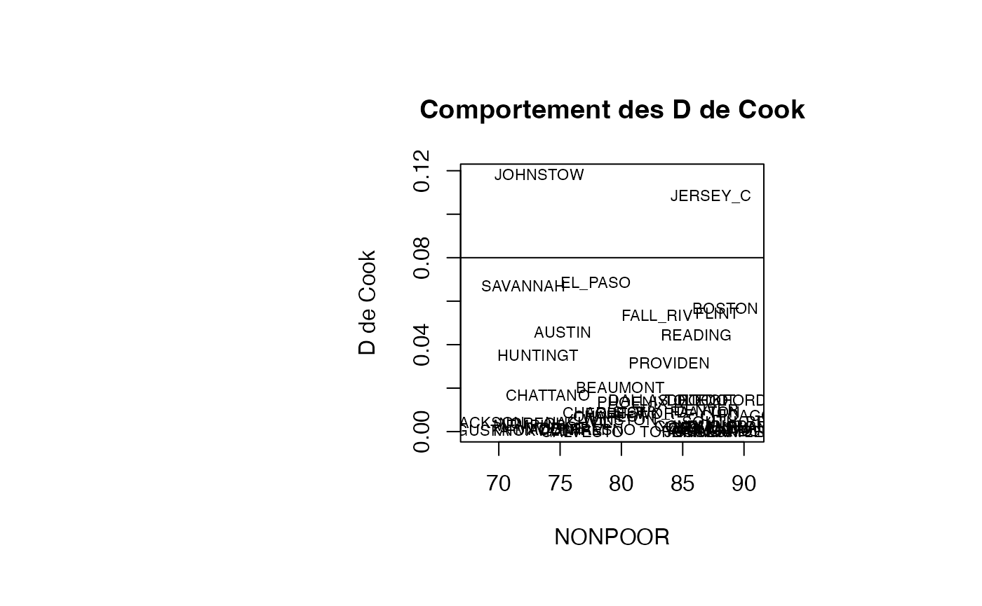

Analyse du modèle TMR vs PERWH

par(oma=c(0,12,1,5)+1,bg="white")
plot(air_pollution$PERWH, air_pollution$TMR, type = "n",xlab="PERWH",ylab="TMR",main="Evolution de TMR en fonction de PERWH")
text(air_pollution$PERWH, air_pollution$TMR, air_pollution$CITY,col='black',cex=0.7)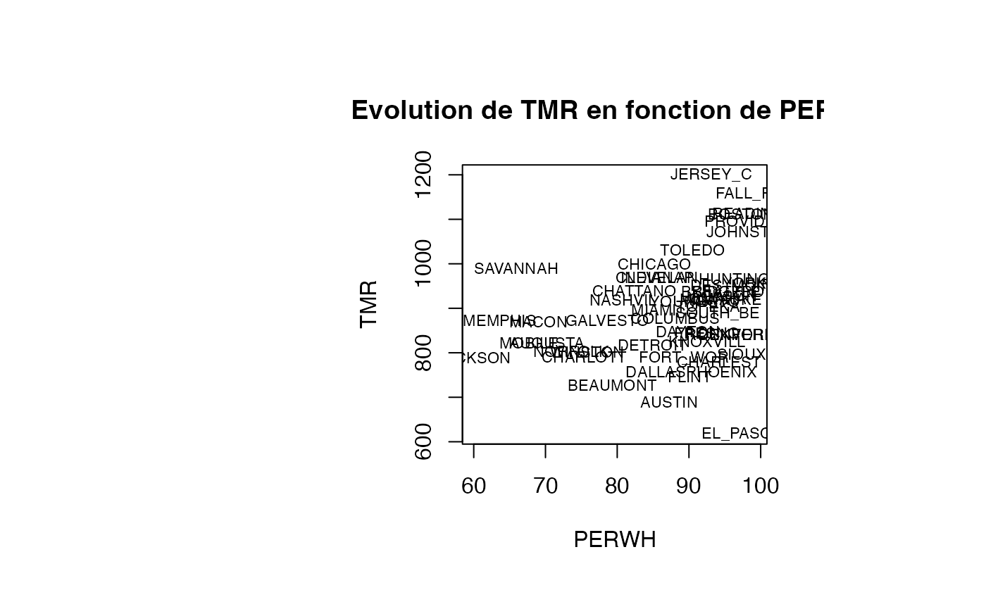

rstudent_leverage <- olsrr::ols_prep_rstudlev_data(reg_TMR_PERWH)
rstudent <- rstudent_leverage$levrstud$rstudent
result_TMR_PERWH <- data.frame(air_pollution,rstudent)
par(oma=c(0,12,1,5)+1,bg="white")
plot(result_TMR_PERWH$PERWH, result_TMR_PERWH$rstudent, type = "n",xlab="PERWH",ylab="RStudents",main="Comportement des RStudents")
text(result_TMR_PERWH$PERWH, result_TMR_PERWH$rstudent, result_TMR_PERWH$CITY,col='black',cex=0.7)
abline(h=c(-1.99,0,1.99))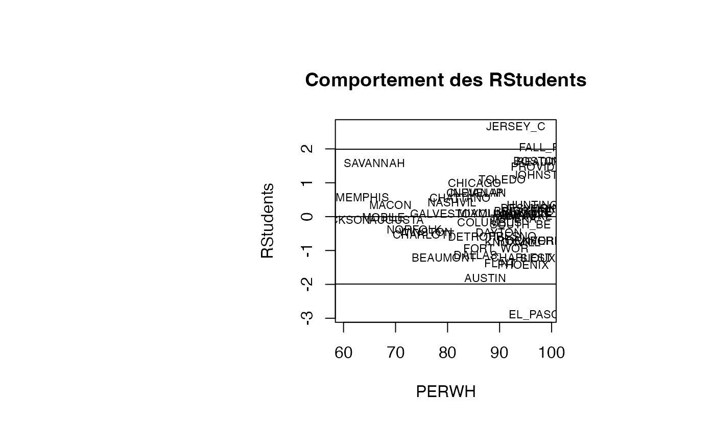

leverage <- rstudent_leverage$levrstud$leverage
result_TMR_PERWH <- data.frame(result_TMR_PERWH,leverage)
par(oma=c(0,12,1,5)+1,bg="white")
plot(result_TMR_PERWH$PERWH, result_TMR_PERWH$leverage, type = "n",xlab="PERWH",ylab="Levier",main="Comportement des leviers")
text(result_TMR_PERWH$PERWH, result_TMR_PERWH$leverage, result_TMR_PERWH$CITY,col='black',cex=0.7)
abline(h=0.08)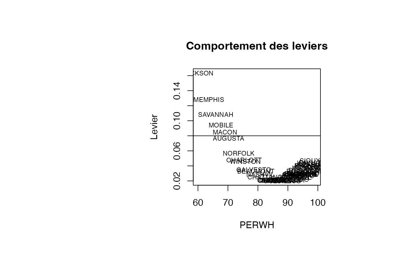

resid <- reg_TMR_PERWH$residuals
rmse <- sqrt(49*var(resid)/48)
resid_std <- resid/rmse

cookd <- matrix(0,nrow=50)
for (i in 1:50)
    {cookd[i]=(leverage[i]/(1-leverage[i]))*(resid_std[i]^2/(2*(1-leverage[i])))}
result_TMR_PERWH <- data.frame(result_TMR_PERWH,cookd)
par(oma=c(0,12,1,5)+1,bg="white")
plot(result_TMR_PERWH$PERWH, result_TMR_PERWH$cookd, type = "n",xlab="PERWH",ylab="D de Cook",main="Comportement des D de Cook")
text(result_TMR_PERWH$PERWH, result_TMR_PERWH$cookd, result_TMR_PERWH$CITY,col='black',cex=0.7)
abline(h=0.08)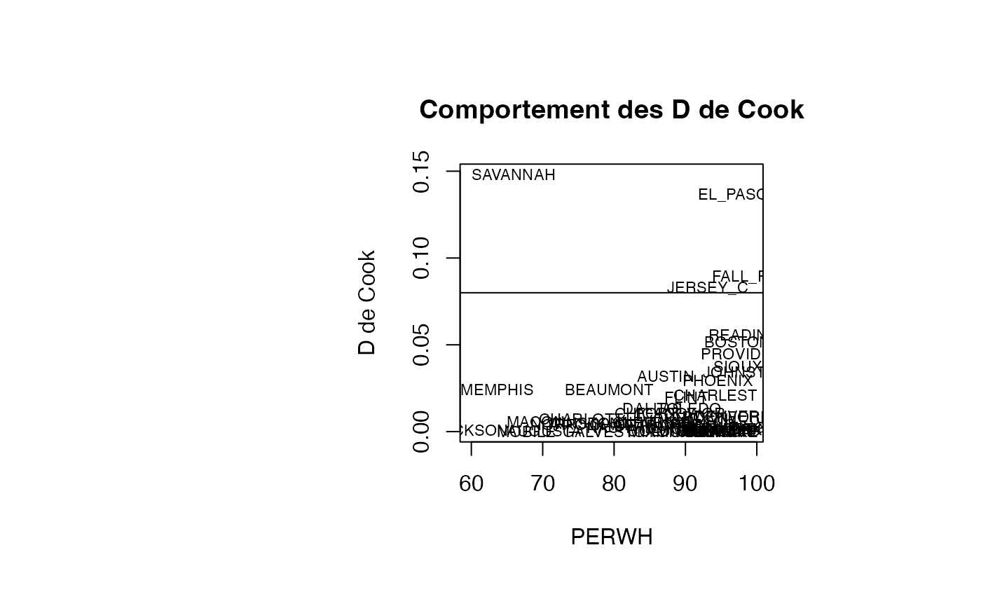

Exercices 10.4 : Intervalles de confiance et de prévision

Analyse du modèle TMR vs GE65

IC_95 <- predict(reg_TMR_GE65, interval="confidence")
IC_95 <- data.frame(IC_95)
binf_IC_95 <- IC_95$lwr
bsup_IC_95 <- IC_95$upr
result_TMR_GE65 <- data.frame(air_pollution,binf_IC_95,bsup_IC_95)
par(oma=c(0,12,1,5)+1,bg="white")
plot(air_pollution$GE65, air_pollution$TMR, type = "p",xlab="GE65",ylab="TMR")
abline(reg_TMR_GE65)
matlines(result_TMR_GE65$GE65,IC_95[,2:3],lty=c(2,2),col="black")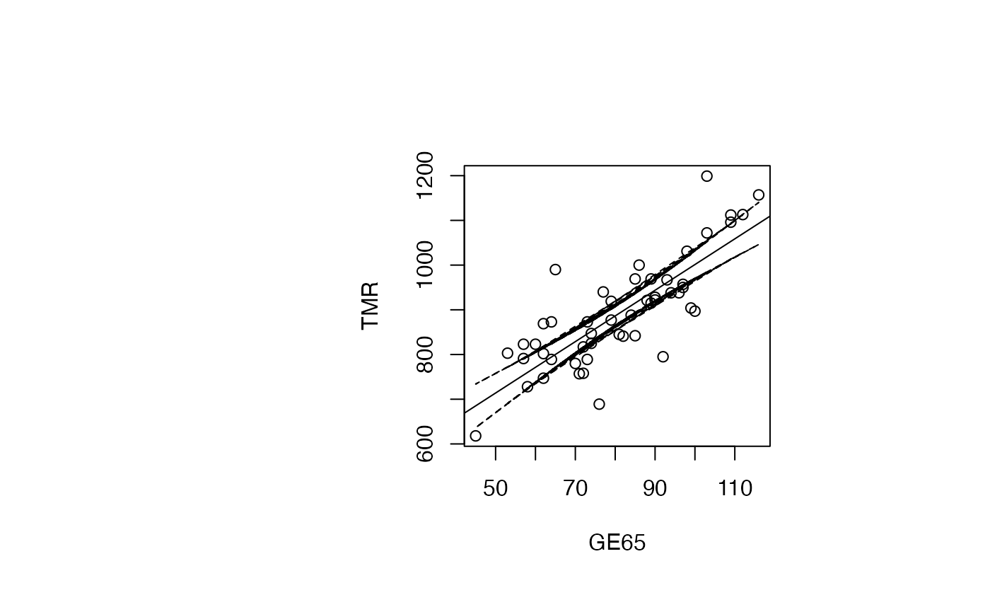

IP_95 <- predict(reg_TMR_GE65, interval="prediction")
#> Warning in predict.lm(reg_TMR_GE65, interval = "prediction"): predictions on current data refer to _future_ responses
IP_95 <- data.frame(IP_95)
binf_IP_95 <- IP_95$lwr
bsup_IP_95 <- IP_95$upr
result_TMR_GE65 <- data.frame(result_TMR_GE65,binf_IP_95,bsup_IP_95)
par(oma=c(0,12,1,5)+1,bg="white")
plot(air_pollution$GE65, air_pollution$TMR, type = "n",xlab="GE65",ylab="TMR")
text(air_pollution$GE65, air_pollution$TMR, air_pollution$CITY,col='black',cex=0.7)
abline(reg_TMR_GE65)
matlines(air_pollution$GE65,IP_95[,2:3],lty=c(2,2),col="black")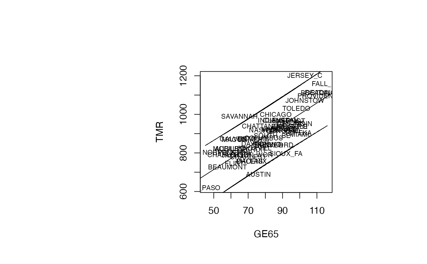

Analyse du modèle TMR vs l_pm2

IC_95 <- predict(reg_TMR_l_pm2, interval="confidence")
IC_95 <- data.frame(IC_95)
binf_IC_95 <- IC_95$lwr
bsup_IC_95 <- IC_95$upr
result_TMR_l_pm2 <- data.frame(air_pollution,binf_IC_95,bsup_IC_95)
par(oma=c(0,12,1,5)+1,bg="white")
plot(air_pollution$l_pm2, air_pollution$TMR, type = "p",xlab="l_pm2",ylab="TMR")
abline(reg_TMR_l_pm2)
matlines(result_TMR_l_pm2$l_pm2,IC_95[,2:3],lty=c(2,2),col="black")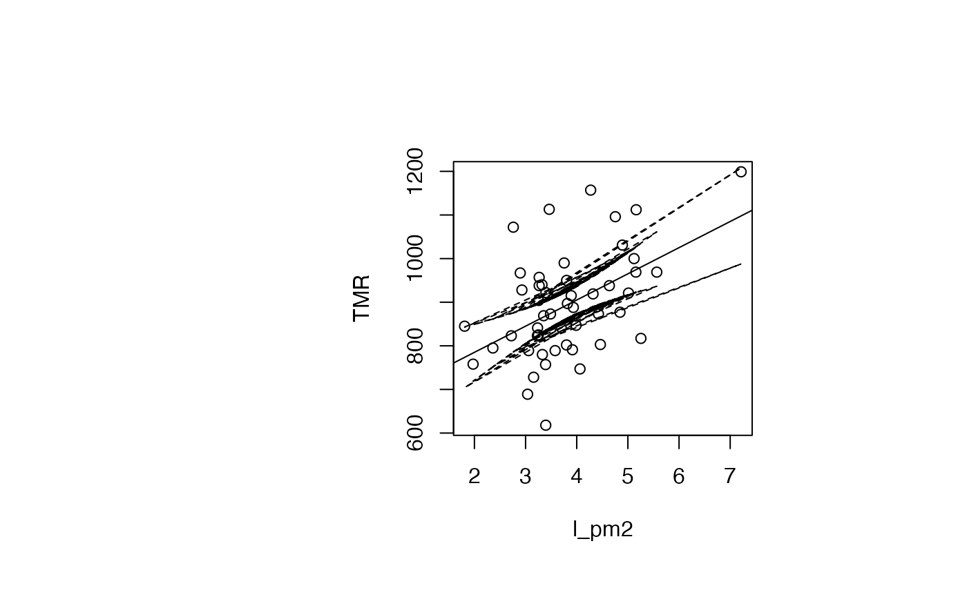

IP_95 <- predict(reg_TMR_l_pm2, interval="prediction")
#> Warning in predict.lm(reg_TMR_l_pm2, interval = "prediction"): predictions on current data refer to _future_ responses
IP_95 <- data.frame(IP_95)
binf_IP_95 <- IP_95$lwr
bsup_IP_95 <- IP_95$upr
result_TMR_l_pm2 <- data.frame(result_TMR_l_pm2,binf_IP_95,bsup_IP_95)
par(oma=c(0,12,1,5)+1,bg="white")
plot(air_pollution$l_pm2, air_pollution$TMR, type = "n",xlab="l_pm2",ylab="TMR")
text(air_pollution$l_pm2, air_pollution$TMR, air_pollution$CITY,col='black',cex=0.7)
abline(reg_TMR_l_pm2)
matlines(air_pollution$l_pm2,IP_95[,2:3],lty=c(2,2),col="black")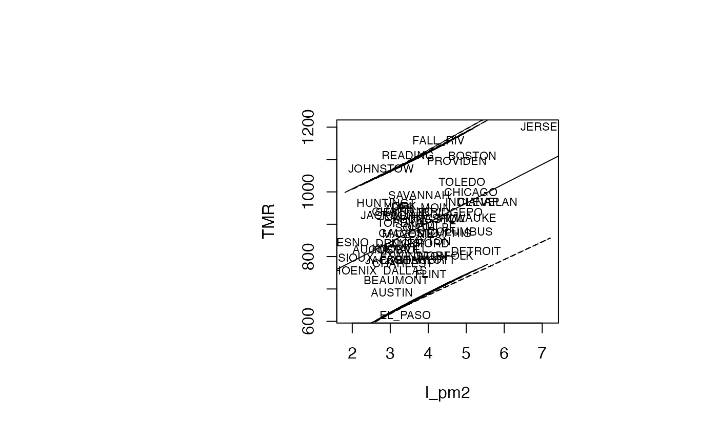

Analyse du modèle TMR vs SMIN

IC_95 <- predict(reg_TMR_SMIN, interval="confidence")
IC_95 <- data.frame(IC_95)
binf_IC_95 <- IC_95$lwr
bsup_IC_95 <- IC_95$upr
result_TMR_SMIN <- data.frame(air_pollution,binf_IC_95,bsup_IC_95)
par(oma=c(0,12,1,5)+1,bg="white")
plot(air_pollution$SMIN, air_pollution$TMR, type = "p",xlab="SMIN",ylab="TMR")
abline(reg_TMR_SMIN)
matlines(result_TMR_SMIN$SMIN,IC_95[,2:3],lty=c(2,2),col="black")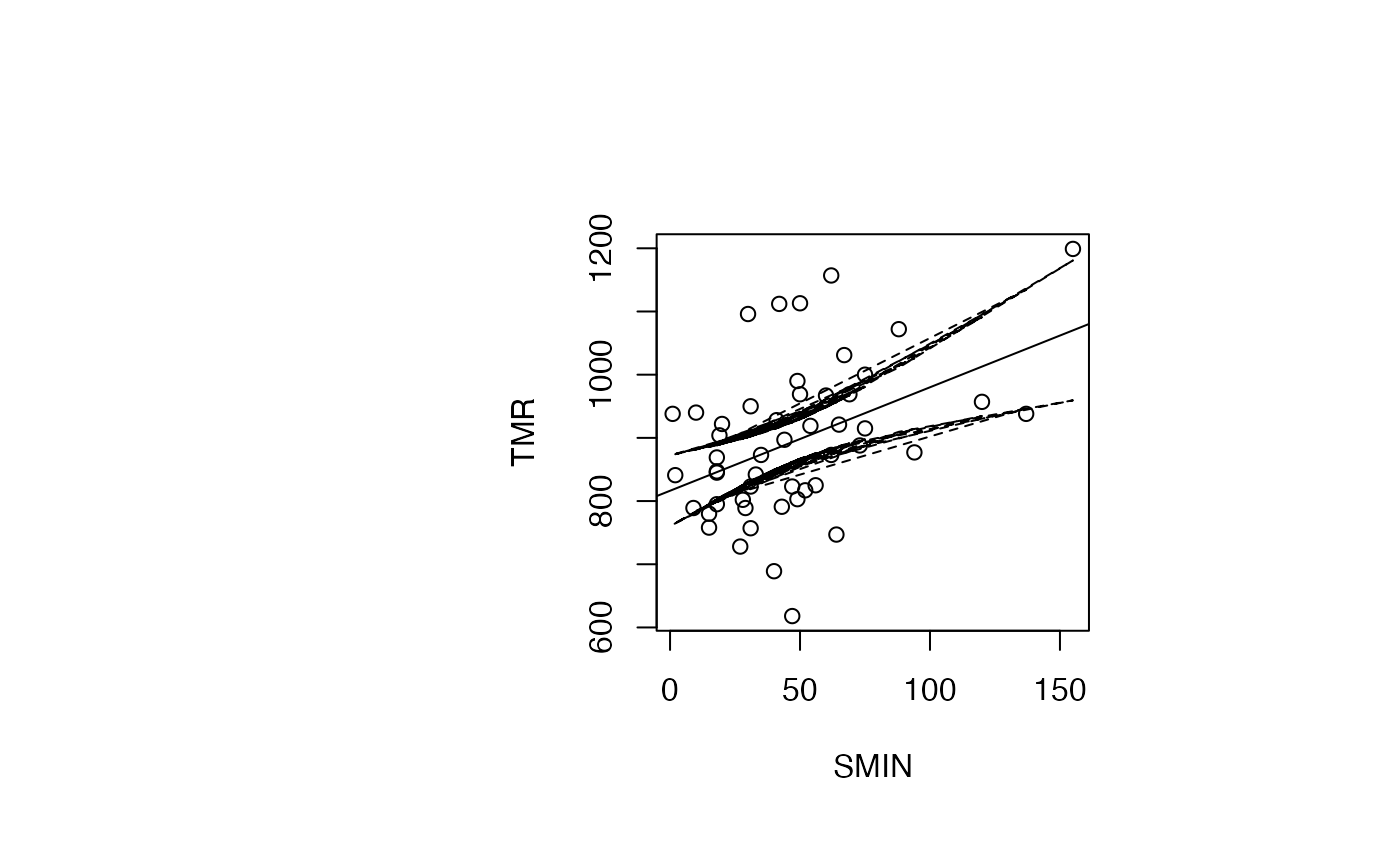

IP_95 <- predict(reg_TMR_SMIN, interval="prediction")
#> Warning in predict.lm(reg_TMR_SMIN, interval = "prediction"): predictions on current data refer to _future_ responses
IP_95 <- data.frame(IP_95)
binf_IP_95 <- IP_95$lwr
bsup_IP_95 <- IP_95$upr
result_TMR_SMIN <- data.frame(result_TMR_SMIN,binf_IP_95,bsup_IP_95)
par(oma=c(0,12,1,5)+1,bg="white")
plot(air_pollution$SMIN, air_pollution$TMR, type = "n",xlab="SMIN",ylab="TMR")
text(air_pollution$SMIN, air_pollution$TMR, air_pollution$CITY,col='black',cex=0.7)
abline(reg_TMR_SMIN)
matlines(air_pollution$SMIN,IP_95[,2:3],lty=c(2,2),col="black")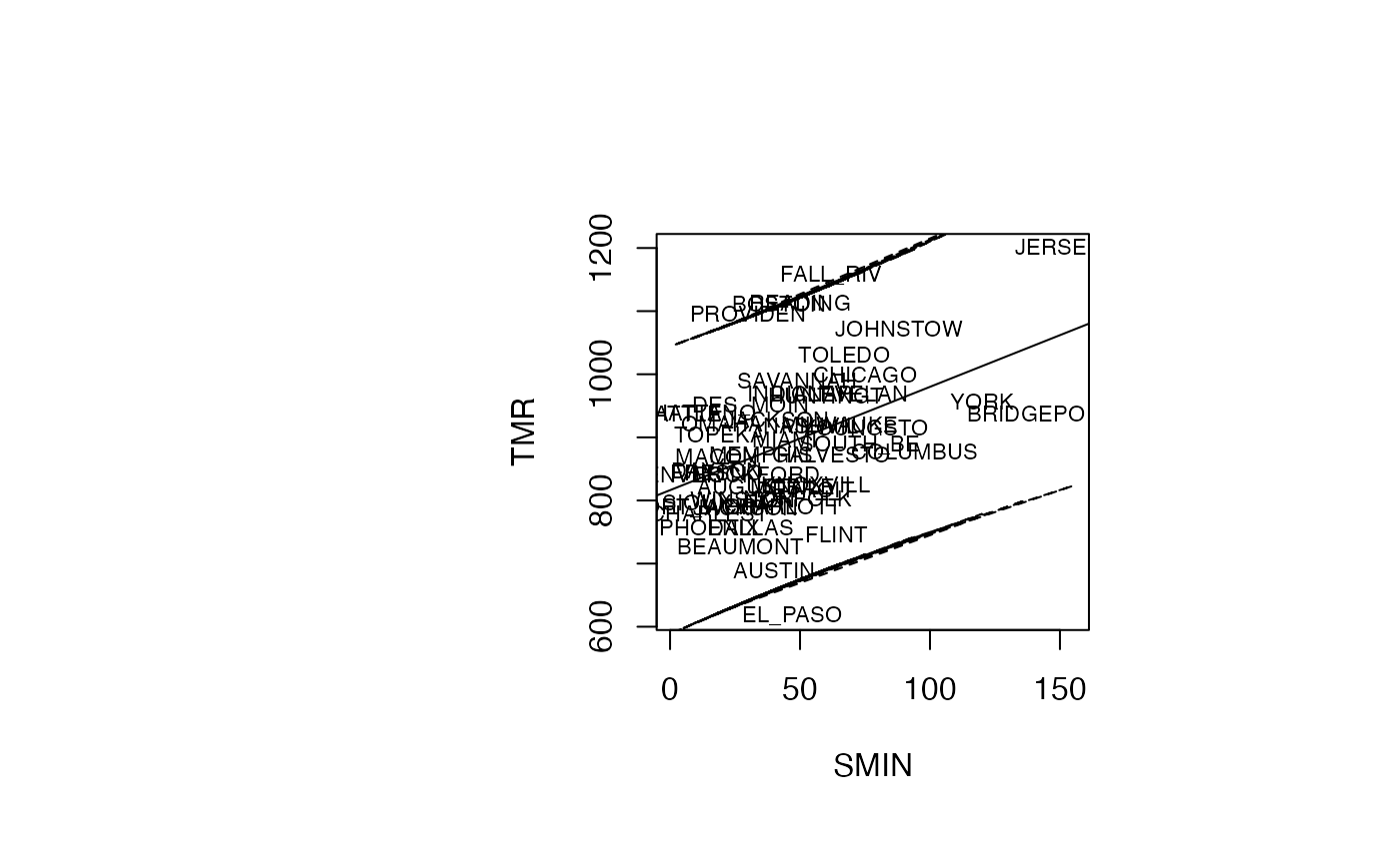

Analyse du modèle TMR vs SMEAN

IC_95 <- predict(reg_TMR_SMEAN, interval="confidence")
IC_95 <- data.frame(IC_95)
binf_IC_95 <- IC_95$lwr
bsup_IC_95 <- IC_95$upr
result_TMR_SMEAN <- data.frame(air_pollution,binf_IC_95,bsup_IC_95)
par(oma=c(0,12,1,5)+1,bg="white")
plot(air_pollution$SMEAN, air_pollution$TMR, type = "p",xlab="SMEAN",ylab="TMR")
abline(reg_TMR_SMEAN)
matlines(result_TMR_SMEAN$SMEAN,IC_95[,2:3],lty=c(2,2),col="black")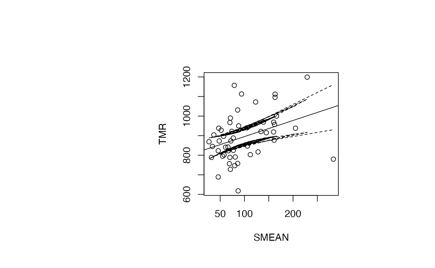

IP_95 <- predict(reg_TMR_SMEAN, interval="prediction")
#> Warning in predict.lm(reg_TMR_SMEAN, interval = "prediction"): predictions on current data refer to _future_ responses
IP_95 <- data.frame(IP_95)
binf_IP_95 <- IP_95$lwr
bsup_IP_95 <- IP_95$upr
result_TMR_SMEAN <- data.frame(result_TMR_SMEAN,binf_IP_95,bsup_IP_95)
par(oma=c(0,12,1,5)+1,bg="white")
plot(air_pollution$SMEAN, air_pollution$TMR, type = "n",xlab="SMEAN",ylab="TMR")
text(air_pollution$SMEAN, air_pollution$TMR, air_pollution$CITY,col='black',cex=0.7)
abline(reg_TMR_SMEAN)
matlines(air_pollution$SMEAN,IP_95[,2:3],lty=c(2,2),col="black")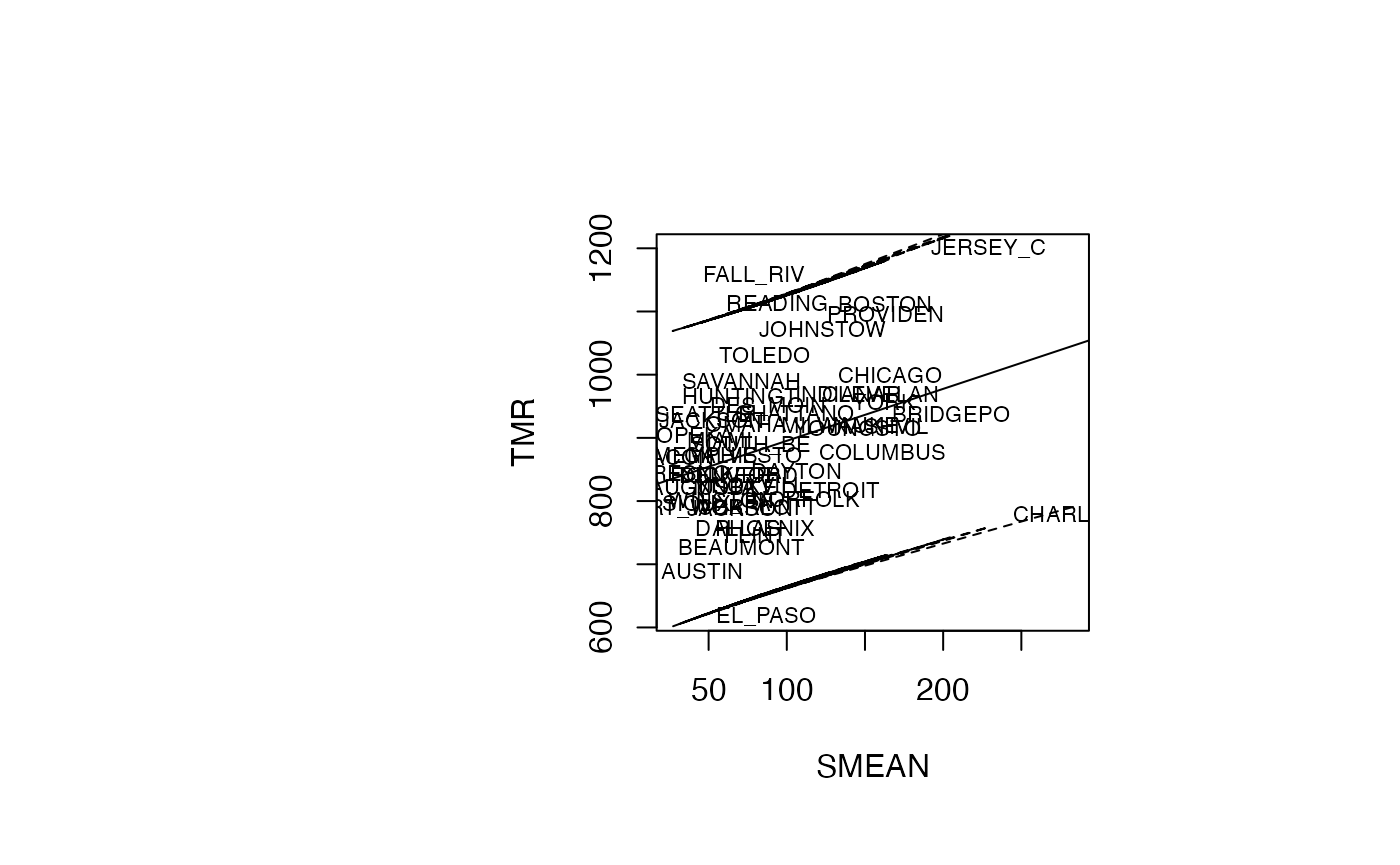

Analyse du modèle TMR vs NONPOOR

IC_95 <- predict(reg_TMR_NONPOOR, interval="confidence")
IC_95 <- data.frame(IC_95)
binf_IC_95 <- IC_95$lwr
bsup_IC_95 <- IC_95$upr
result_TMR_NONPOOR <- data.frame(air_pollution,binf_IC_95,bsup_IC_95)
par(oma=c(0,12,1,5)+1,bg="white")
plot(air_pollution$NONPOOR, air_pollution$TMR, type = "p",xlab="NONPOOR",ylab="TMR")
abline(reg_TMR_NONPOOR)
matlines(result_TMR_NONPOOR$NONPOOR,IC_95[,2:3],lty=c(2,2),col="black")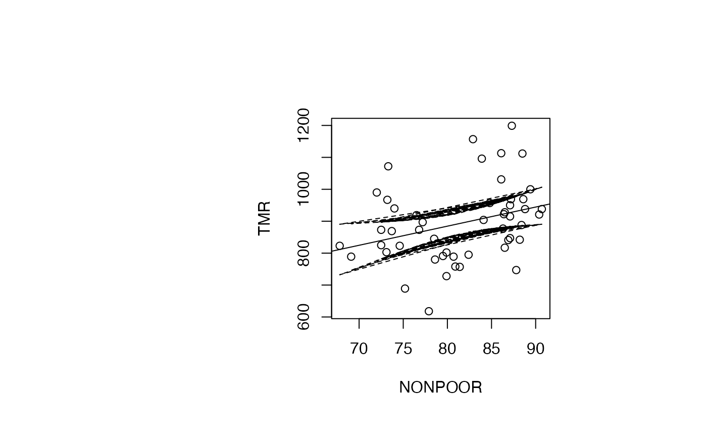

IP_95 <- predict(reg_TMR_NONPOOR, interval="prediction")
#> Warning in predict.lm(reg_TMR_NONPOOR, interval = "prediction"): predictions on current data refer to _future_ responses
IP_95 <- data.frame(IP_95)
binf_IP_95 <- IP_95$lwr
bsup_IP_95 <- IP_95$upr
result_TMR_NONPOOR <- data.frame(result_TMR_NONPOOR,binf_IP_95,bsup_IP_95)
par(oma=c(0,12,1,5)+1,bg="white")
plot(air_pollution$NONPOOR, air_pollution$TMR, type = "n",xlab="NONPOOR",ylab="TMR")
text(air_pollution$NONPOOR, air_pollution$TMR, air_pollution$CITY,col='black',cex=0.7)
abline(reg_TMR_NONPOOR)
matlines(air_pollution$NONPOOR,IP_95[,2:3],lty=c(2,2),col="black")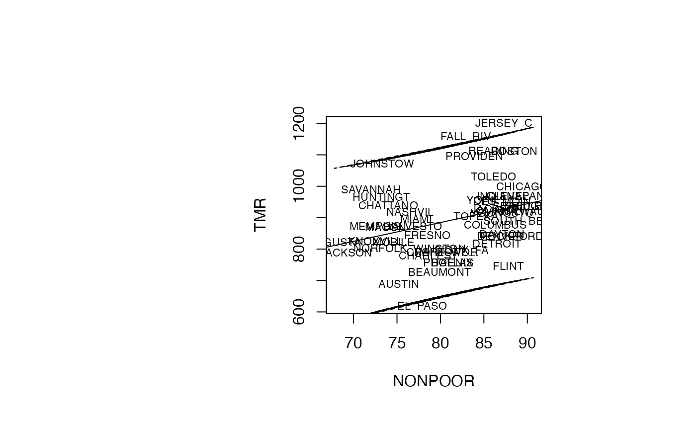

Analyse du modèle TMR vs PERWH

IC_95 <- predict(reg_TMR_PERWH, interval="confidence")
IC_95 <- data.frame(IC_95)
binf_IC_95 <- IC_95$lwr
bsup_IC_95 <- IC_95$upr
result_TMR_PERWH <- data.frame(air_pollution,binf_IC_95,bsup_IC_95)
par(oma=c(0,12,1,5)+1,bg="white")
plot(air_pollution$PERWH, air_pollution$TMR, type = "p",xlab="PERWH",ylab="TMR")
abline(reg_TMR_PERWH)
matlines(result_TMR_PERWH$PERWH,IC_95[,2:3],lty=c(2,2),col="black")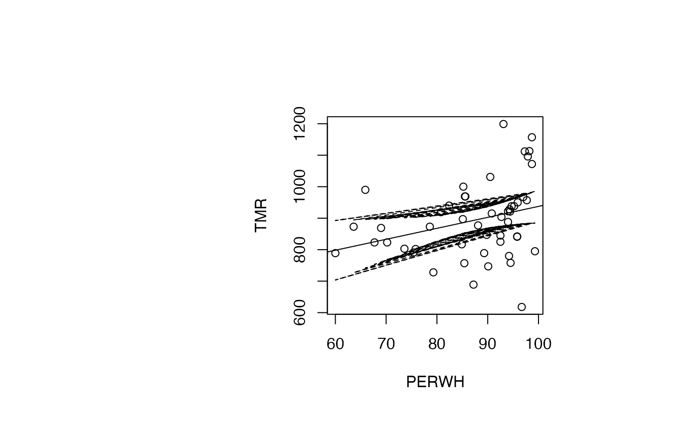

IP_95 <- predict(reg_TMR_PERWH, interval="prediction")
#> Warning in predict.lm(reg_TMR_PERWH, interval = "prediction"): predictions on current data refer to _future_ responses
IP_95 <- data.frame(IP_95)
binf_IP_95 <- IP_95$lwr
bsup_IP_95 <- IP_95$upr
result_TMR_PERWH <- data.frame(result_TMR_PERWH,binf_IP_95,bsup_IP_95)
par(oma=c(0,12,1,5)+1,bg="white")
plot(air_pollution$PERWH, air_pollution$TMR, type = "n",xlab="PERWH",ylab="TMR")
text(air_pollution$PERWH, air_pollution$TMR, air_pollution$CITY,col='black',cex=0.7)
abline(reg_TMR_PERWH)
matlines(air_pollution$PERWH,IP_95[,2:3],lty=c(2,2),col="black")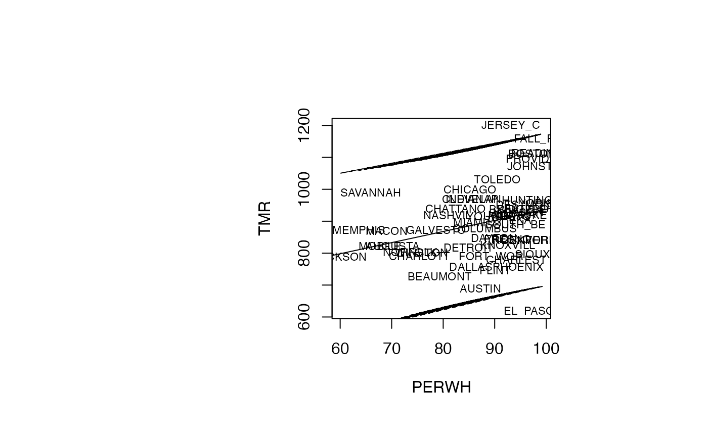

Exercice 10.5 : Régression multiple

reg_TMR_all <- lm(TMR~SMIN+SMEAN+SMAX+PMIN+PMEAN+PERWH+NONPOOR+GE65+LPOP+l_pm2+l_pmax,data=air_pollution)
summary(reg_TMR_all)
#> 
#> Call:
#> lm(formula = TMR ~ SMIN + SMEAN + SMAX + PMIN + PMEAN + PERWH + 
#>     NONPOOR + GE65 + LPOP + l_pm2 + l_pmax, data = air_pollution)
#> 
#> Residuals:
#>      Min       1Q   Median       3Q      Max 
#> -123.570  -23.858    4.477   32.310  104.264 
#> 
#> Coefficients:
#>              Estimate Std. Error t value Pr(>|t|)    
#> (Intercept) 601.67911  243.89675   2.467   0.0182 *  
#> SMIN          0.39119    0.36334   1.077   0.2884    
#> SMEAN        -0.21686    0.45596  -0.476   0.6371    
#> SMAX          0.07739    0.14112   0.548   0.5866    
#> PMIN          1.10963    0.76616   1.448   0.1557    
#> PMEAN        -0.40629    0.58083  -0.699   0.4885    
#> PERWH        -3.13718    1.41835  -2.212   0.0331 *  
#> NONPOOR      -3.21879    2.08732  -1.542   0.1313    
#> GE65          7.15451    0.67558  10.590 6.77e-13 ***
#> LPOP        -24.30248   27.95434  -0.869   0.3901    
#> l_pm2        36.78162   16.01267   2.297   0.0272 *  
#> l_pmax       41.24149   36.44439   1.132   0.2649    
#> ---
#> Signif. codes:  0 '***' 0.001 '**' 0.01 '*' 0.05 '.' 0.1 ' ' 1
#> 
#> Residual standard error: 53.91 on 38 degrees of freedom
#> Multiple R-squared:  0.845,  Adjusted R-squared:  0.8001 
#> F-statistic: 18.83 on 11 and 38 DF,  p-value: 3.998e-12

Exercice 10.6 : Régression simplifié

reg_TMR_simplifie <- lm(TMR~PERWH+GE65+l_pm2,data=air_pollution)
summary(reg_TMR_simplifie)
#> 
#> Call:
#> lm(formula = TMR ~ PERWH + GE65 + l_pm2, data = air_pollution)
#> 
#> Residuals:
#>      Min       1Q   Median       3Q      Max 
#> -146.219  -29.145    3.364   29.679  126.272 
#> 
#> Coefficients:
#>             Estimate Std. Error t value Pr(>|t|)    
#> (Intercept) 560.0295    77.3237   7.243 3.95e-09 ***
#> PERWH        -3.8830     1.0515  -3.693 0.000587 ***
#> GE65          6.8760     0.6657  10.329 1.44e-13 ***
#> l_pm2        30.0058     8.6584   3.466 0.001157 ** 
#> ---
#> Signif. codes:  0 '***' 0.001 '**' 0.01 '*' 0.05 '.' 0.1 ' ' 1
#> 
#> Residual standard error: 55.94 on 46 degrees of freedom
#> Multiple R-squared:  0.798,  Adjusted R-squared:  0.7848 
#> F-statistic: 60.56 on 3 and 46 DF,  p-value: 5.232e-16

Exercice 10.7 : Régression multiple par sélection de variables

Définir la graine aléatoire pour pouvoir reproduire les simulations

set.seed(123)

Mise en place de la validation croisée \(k\)-fold

train.control <- caret::trainControl(method = "cv", number = 10)

Sélection ascendante

step.model <- caret::train(TMR~SMIN+SMEAN+SMAX+PMIN+PMEAN+PERWH+NONPOOR+GE65+LPOP+l_pm2+l_pmax,data=air_pollution,method = "leapForward", tuneGrid = data.frame(nvmax = 1:5), trControl = train.control)
step.model$results
#>   nvmax     RMSE  Rsquared      MAE   RMSESD RsquaredSD    MAESD
#> 1     1 69.18548 0.6759393 56.67012 21.96414 0.18841443 16.08476
#> 2     2 65.10777 0.7115294 47.56491 20.32729 0.13930059 14.28262
#> 3     3 59.58531 0.7737680 47.64129 13.08864 0.09672402 11.05144
#> 4     4 63.39414 0.7345135 51.43794 15.85645 0.14911173 15.58864
#> 5     5 59.80585 0.7610921 48.97589 17.25668 0.15858671 13.81363

step.model$bestTune
#>   nvmax
#> 3     3

summary(step.model$finalModel)
#> Subset selection object
#> 11 Variables  (and intercept)
#>         Forced in Forced out
#> SMIN        FALSE      FALSE
#> SMEAN       FALSE      FALSE
#> SMAX        FALSE      FALSE
#> PMIN        FALSE      FALSE
#> PMEAN       FALSE      FALSE
#> PERWH       FALSE      FALSE
#> NONPOOR     FALSE      FALSE
#> GE65        FALSE      FALSE
#> LPOP        FALSE      FALSE
#> l_pm2       FALSE      FALSE
#> l_pmax      FALSE      FALSE
#> 1 subsets of each size up to 3
#> Selection Algorithm: forward
#>          SMIN SMEAN SMAX PMIN PMEAN PERWH NONPOOR GE65 LPOP l_pm2 l_pmax
#> 1  ( 1 ) " "  " "   " "  " "  " "   " "   " "     "*"  " "  " "   " "   
#> 2  ( 1 ) " "  " "   " "  " "  " "   "*"   " "     "*"  " "  " "   " "   
#> 3  ( 1 ) " "  " "   " "  " "  " "   "*"   " "     "*"  " "  "*"   " "

reg_TMR_forward <- lm(TMR~PERWH+GE65+l_pm2,data=air_pollution)
summary(reg_TMR_forward)
#> 
#> Call:
#> lm(formula = TMR ~ PERWH + GE65 + l_pm2, data = air_pollution)
#> 
#> Residuals:
#>      Min       1Q   Median       3Q      Max 
#> -146.219  -29.145    3.364   29.679  126.272 
#> 
#> Coefficients:
#>             Estimate Std. Error t value Pr(>|t|)    
#> (Intercept) 560.0295    77.3237   7.243 3.95e-09 ***
#> PERWH        -3.8830     1.0515  -3.693 0.000587 ***
#> GE65          6.8760     0.6657  10.329 1.44e-13 ***
#> l_pm2        30.0058     8.6584   3.466 0.001157 ** 
#> ---
#> Signif. codes:  0 '***' 0.001 '**' 0.01 '*' 0.05 '.' 0.1 ' ' 1
#> 
#> Residual standard error: 55.94 on 46 degrees of freedom
#> Multiple R-squared:  0.798,  Adjusted R-squared:  0.7848 
#> F-statistic: 60.56 on 3 and 46 DF,  p-value: 5.232e-16

Sélection descendante

step.model <- caret::train(TMR~SMIN+SMEAN+SMAX+PMIN+PMEAN+PERWH+NONPOOR+GE65+LPOP+l_pm2+l_pmax,data=air_pollution, method = "leapBackward", tuneGrid = data.frame(nvmax = 1:5), trControl = train.control)
step.model$results
#>   nvmax     RMSE  Rsquared      MAE   RMSESD RsquaredSD    MAESD
#> 1     1 70.09854 0.6630928 58.32681 26.56512  0.3333468 18.82932
#> 2     2 70.79554 0.6879672 59.56725 33.02547  0.3136828 29.16886
#> 3     3 60.04721 0.7486923 50.28272 28.11412  0.2589395 24.67720
#> 4     4 63.88906 0.7018427 53.05051 25.87602  0.3000792 22.71978
#> 5     5 66.69164 0.6917069 53.66172 22.19340  0.2961117 21.90087

step.model$bestTune
#>   nvmax
#> 3     3

summary(step.model$finalModel)
#> Subset selection object
#> 11 Variables  (and intercept)
#>         Forced in Forced out
#> SMIN        FALSE      FALSE
#> SMEAN       FALSE      FALSE
#> SMAX        FALSE      FALSE
#> PMIN        FALSE      FALSE
#> PMEAN       FALSE      FALSE
#> PERWH       FALSE      FALSE
#> NONPOOR     FALSE      FALSE
#> GE65        FALSE      FALSE
#> LPOP        FALSE      FALSE
#> l_pm2       FALSE      FALSE
#> l_pmax      FALSE      FALSE
#> 1 subsets of each size up to 3
#> Selection Algorithm: backward
#>          SMIN SMEAN SMAX PMIN PMEAN PERWH NONPOOR GE65 LPOP l_pm2 l_pmax
#> 1  ( 1 ) " "  " "   " "  " "  " "   " "   " "     "*"  " "  " "   " "   
#> 2  ( 1 ) " "  " "   " "  " "  " "   " "   " "     "*"  " "  "*"   " "   
#> 3  ( 1 ) " "  " "   " "  " "  " "   " "   "*"     "*"  " "  "*"   " "

reg_TMR_backward <- lm(TMR~NONPOOR+GE65+l_pm2,data=air_pollution)
summary(reg_TMR_backward)
#> 
#> Call:
#> lm(formula = TMR ~ NONPOOR + GE65 + l_pm2, data = air_pollution)
#> 
#> Residuals:
#>      Min       1Q   Median       3Q      Max 
#> -170.356  -28.518    3.817   30.665  142.149 
#> 
#> Coefficients:
#>             Estimate Std. Error t value Pr(>|t|)    
#> (Intercept) 685.4547   105.3949   6.504 5.07e-08 ***
#> NONPOOR      -5.9609     1.5899  -3.749 0.000494 ***
#> GE65          6.1259     0.5447  11.246 8.55e-15 ***
#> l_pm2        51.5150     9.1878   5.607 1.12e-06 ***
#> ---
#> Signif. codes:  0 '***' 0.001 '**' 0.01 '*' 0.05 '.' 0.1 ' ' 1
#> 
#> Residual standard error: 55.74 on 46 degrees of freedom
#> Multiple R-squared:  0.7994, Adjusted R-squared:  0.7863 
#> F-statistic: 61.09 on 3 and 46 DF,  p-value: 4.455e-16

Sélection pas à pas

step.model <- caret::train(TMR~SMIN+SMEAN+SMAX+PMIN+PMEAN+PERWH+NONPOOR+GE65+LPOP+l_pm2+l_pmax,data=air_pollution, method = "leapSeq",tuneGrid = data.frame(nvmax = 1:5), trControl = train.control)
step.model$results
#>   nvmax     RMSE  Rsquared      MAE   RMSESD RsquaredSD    MAESD
#> 1     1 65.32693 0.7683791 55.80282 29.65039  0.2515142 24.60868
#> 2     2 68.55816 0.7503571 53.88524 21.35529  0.2029516 16.01007
#> 3     3 63.78007 0.7537507 50.13378 21.31510  0.1752168 17.63727
#> 4     4 68.42619 0.7092096 58.30839 32.09439  0.2530411 31.49394
#> 5     5 85.12890 0.6197462 68.70314 36.71849  0.2816074 25.49105

step.model$bestTune
#>   nvmax
#> 3     3

summary(step.model$finalModel)
#> Subset selection object
#> 11 Variables  (and intercept)
#>         Forced in Forced out
#> SMIN        FALSE      FALSE
#> SMEAN       FALSE      FALSE
#> SMAX        FALSE      FALSE
#> PMIN        FALSE      FALSE
#> PMEAN       FALSE      FALSE
#> PERWH       FALSE      FALSE
#> NONPOOR     FALSE      FALSE
#> GE65        FALSE      FALSE
#> LPOP        FALSE      FALSE
#> l_pm2       FALSE      FALSE
#> l_pmax      FALSE      FALSE
#> 1 subsets of each size up to 3
#> Selection Algorithm: 'sequential replacement'
#>          SMIN SMEAN SMAX PMIN PMEAN PERWH NONPOOR GE65 LPOP l_pm2 l_pmax
#> 1  ( 1 ) " "  " "   " "  " "  " "   " "   " "     "*"  " "  " "   " "   
#> 2  ( 1 ) " "  " "   " "  " "  " "   "*"   " "     "*"  " "  " "   " "   
#> 3  ( 1 ) " "  " "   " "  " "  " "   " "   "*"     "*"  " "  "*"   " "

reg_TMR_step_by_step <- lm(TMR~NONPOOR+GE65+l_pm2,data=air_pollution)
summary(reg_TMR_step_by_step)
#> 
#> Call:
#> lm(formula = TMR ~ NONPOOR + GE65 + l_pm2, data = air_pollution)
#> 
#> Residuals:
#>      Min       1Q   Median       3Q      Max 
#> -170.356  -28.518    3.817   30.665  142.149 
#> 
#> Coefficients:
#>             Estimate Std. Error t value Pr(>|t|)    
#> (Intercept) 685.4547   105.3949   6.504 5.07e-08 ***
#> NONPOOR      -5.9609     1.5899  -3.749 0.000494 ***
#> GE65          6.1259     0.5447  11.246 8.55e-15 ***
#> l_pm2        51.5150     9.1878   5.607 1.12e-06 ***
#> ---
#> Signif. codes:  0 '***' 0.001 '**' 0.01 '*' 0.05 '.' 0.1 ' ' 1
#> 
#> Residual standard error: 55.74 on 46 degrees of freedom
#> Multiple R-squared:  0.7994, Adjusted R-squared:  0.7863 
#> F-statistic: 61.09 on 3 and 46 DF,  p-value: 4.455e-16

Exercice 10.8 : Analyse des résidus et des observations

reg_TMR_sel <- lm(TMR~PERWH+GE65+l_pm2,data=air_pollution)
summary(reg_TMR_sel)
#> 
#> Call:
#> lm(formula = TMR ~ PERWH + GE65 + l_pm2, data = air_pollution)
#> 
#> Residuals:
#>      Min       1Q   Median       3Q      Max 
#> -146.219  -29.145    3.364   29.679  126.272 
#> 
#> Coefficients:
#>             Estimate Std. Error t value Pr(>|t|)    
#> (Intercept) 560.0295    77.3237   7.243 3.95e-09 ***
#> PERWH        -3.8830     1.0515  -3.693 0.000587 ***
#> GE65          6.8760     0.6657  10.329 1.44e-13 ***
#> l_pm2        30.0058     8.6584   3.466 0.001157 ** 
#> ---
#> Signif. codes:  0 '***' 0.001 '**' 0.01 '*' 0.05 '.' 0.1 ' ' 1
#> 
#> Residual standard error: 55.94 on 46 degrees of freedom
#> Multiple R-squared:  0.798,  Adjusted R-squared:  0.7848 
#> F-statistic: 60.56 on 3 and 46 DF,  p-value: 5.232e-16

resid <- reg_TMR_sel$residuals
pred <- fitted(reg_TMR_sel)

rmse <- sqrt(49*var(resid)/46)
resid_std <- resid/rmse

par(oma=c(0,12,1,5)+1,bg="white")
plot(pred, resid_std, type = "n",xlab="TMR prédit",ylab="Résidus standardisés",main="Comportement des résidus standardisés")
text(pred, resid_std, air_pollution$CITY,col='black',cex=0.7)
abline(h=c(-2,0,2))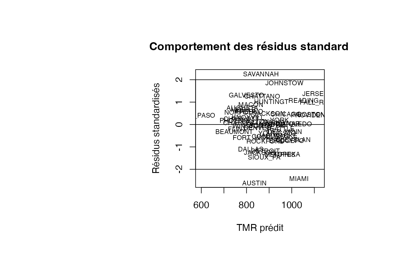

rstudent_leverage <- olsrr::ols_prep_rstudlev_data(reg_TMR_sel)
rstudent <- rstudent_leverage$levrstud$rstudent
result_TMR_sel <- data.frame(air_pollution,rstudent)
par(oma=c(0,12,1,5)+1,bg="white")
plot(pred, result_TMR_sel$rstudent, type = "n",xlab="TMR prédit",ylab="RStudents")
text(pred, result_TMR_sel$rstudent, result_TMR_sel$CITY,col='black',cex=0.7)
abline(h=c(-2.01,0,2.01))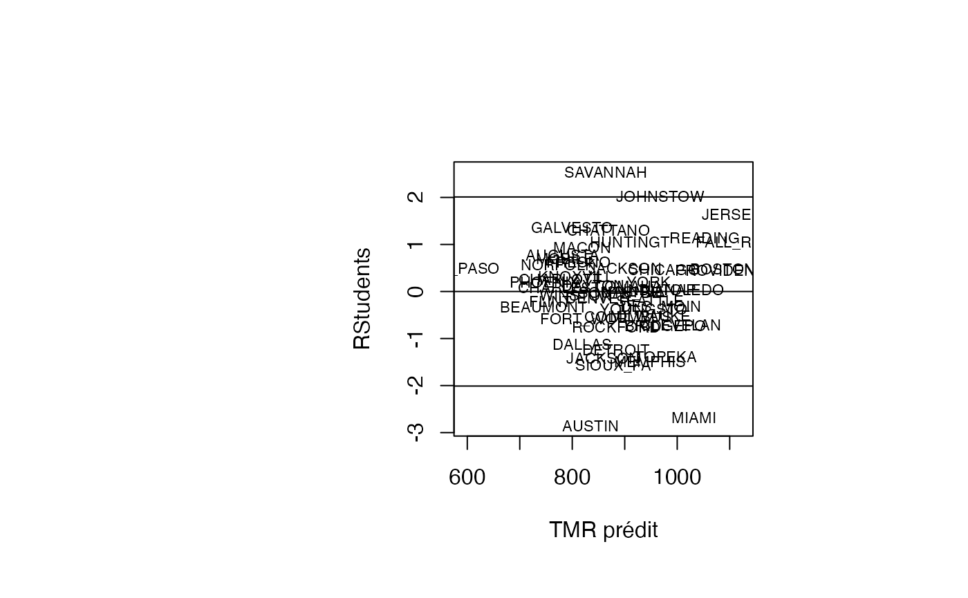

leverage <- rstudent_leverage$levrstud$leverage
result_TMR_sel <- data.frame(result_TMR_sel,leverage)
par(oma=c(0,12,1,5)+1,bg="white")
plot(pred, result_TMR_sel$leverage, type = "n",xlab="TMR prédit",ylab="Leviers")
text(pred, result_TMR_sel$leverage, result_TMR_sel$CITY,col='black',cex=0.7)
abline(h=0.16)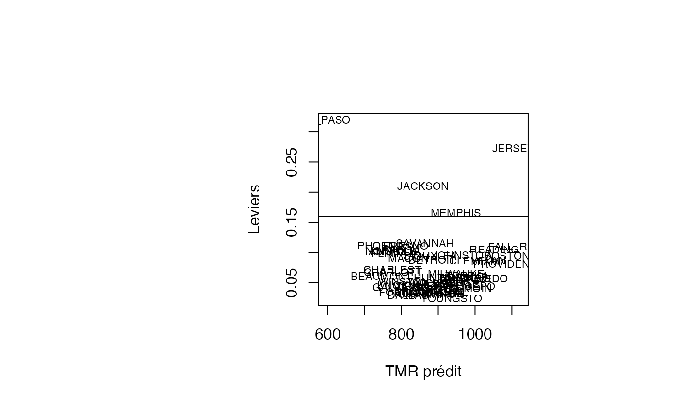

cookd <- matrix(0,nrow=50)
for (i in 1:50)
    {cookd[i]=(leverage[i]/(1-leverage[i]))*(resid_std[i]^2/(2*(1-leverage[i])))}
result_TMR_sel <- data.frame(result_TMR_sel,cookd)
par(oma=c(0,12,1,5)+1,bg="white")
plot(pred, result_TMR_sel$cookd, type = "n",xlab="TMR prédit",ylab="D de Cook")
text(pred, result_TMR_sel$cookd, result_TMR_sel$CITY,col='black',cex=0.7)
abline(h=0.0870)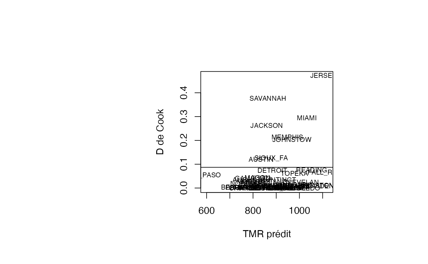

num_ville <- 1:50
dfb <- dfbetas(reg_TMR_sel)
dfbetas <- data.frame(dfb)
dfbetas_GE65 <- dfbetas$GE65
result_TMR_sel <- data.frame(result_TMR_sel,dfbetas_GE65)
dfbetas_l_pm2 <- dfbetas$l_pm2
result_TMR_sel <- data.frame(result_TMR_sel,dfbetas_l_pm2)
dfbetas_PERWH <- dfbetas$PERWH
result_TMR_sel <- data.frame(result_TMR_sel,dfbetas_PERWH)
par(oma=c(0,12,1,5)+1,bg="white")
plot(pred, result_TMR_sel$dfbetas_GE65, type = "n",xlab="TMR prédit",ylab="DFBetas pour GE65")
text(pred, result_TMR_sel$dfbetas_GE65, result_TMR_sel$CITY,col='black',cex=0.7)
abline(h=0.2828)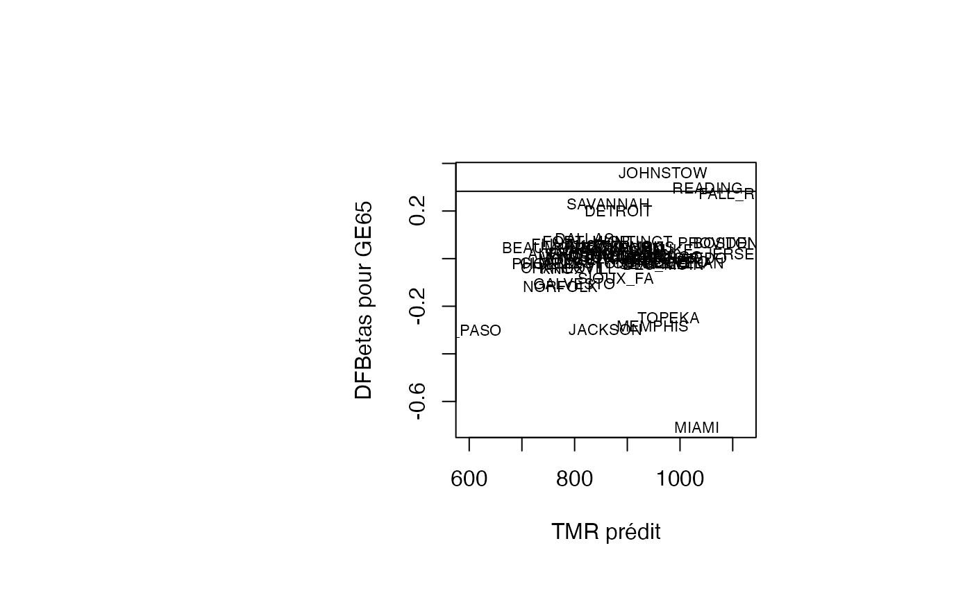

plot(pred, result_TMR_sel$dfbetas_l_pm2, type = "n",xlab="TMR prédit",ylab="DFBetas pour l_pm2")
text(pred, result_TMR_sel$dfbetas_l_pm2, result_TMR_sel$CITY,col='black',cex=0.7)
abline(h=0.2828)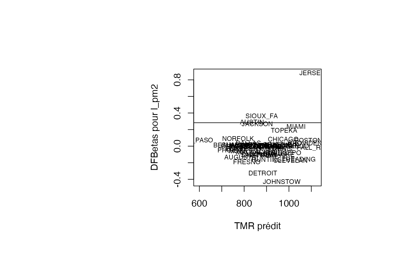

plot(pred, result_TMR_sel$dfbetas_PERWH, type = "n",xlab="TMR prédit",ylab="DFBetas pour PERWH")
text(pred, result_TMR_sel$dfbetas_PERWH, result_TMR_sel$CITY,col='black',cex=0.7)
abline(h=0.2828)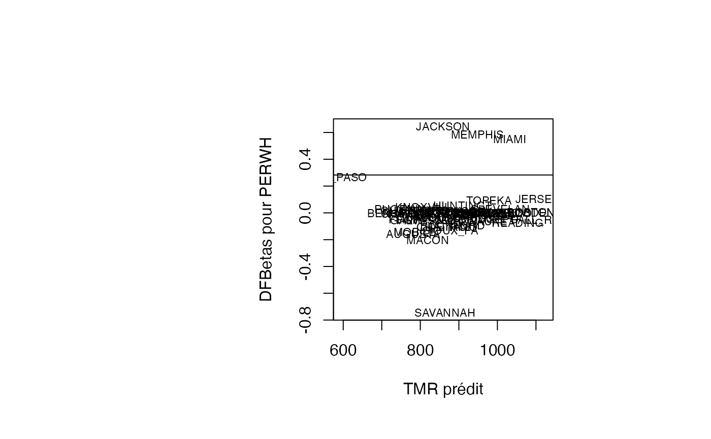

Exercice 10.9 : Intervalles de confiance et de prévision

IC_95 <- predict(reg_TMR_sel, interval="confidence")
IC_95 <- data.frame(IC_95)
binf_IC_95 <- IC_95$lwr
bsup_IC_95 <- IC_95$upr
result_TMR_sel <- data.frame(air_pollution,binf_IC_95,bsup_IC_95)
par(oma=c(0,12,1,5)+1,bg="white")
lattice::xyplot(pred+binf_IC_95+bsup_IC_95~num_ville,type=c("p","l"),lty=1,cex=2,lwd=2,col=c("red","green","green"),xlab="",ylab="TMR")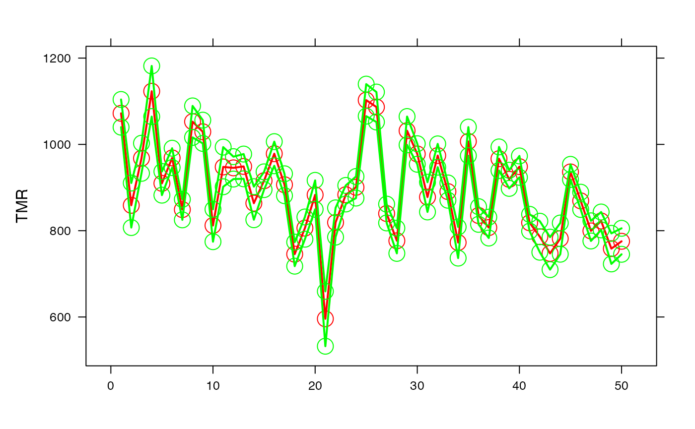

IP_95 <- predict(reg_TMR_sel, interval="prediction")
#> Warning in predict.lm(reg_TMR_sel, interval = "prediction"): predictions on current data refer to _future_ responses
IP_95 <- data.frame(IP_95)
binf_IP_95 <- IP_95$lwr
bsup_IP_95 <- IP_95$upr
result_TMR_sel <- data.frame(result_TMR_sel,binf_IP_95,bsup_IP_95)
par(oma=c(0,12,1,5)+1,bg="white")
lattice::xyplot(air_pollution$TMR+pred+binf_IP_95+bsup_IP_95~num_ville,type=c("p","l"),lty=1,cex=2,lwd=2,col=c("blue","red","green","green"),xlab="",ylab="TMR")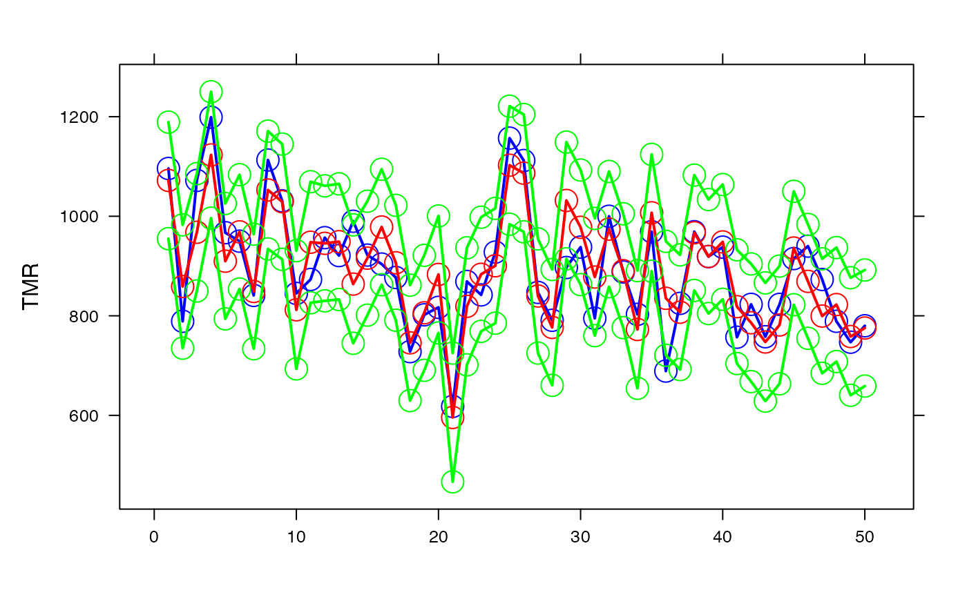

Exercice 10.10 : Multicolinéarité

Modèle avec GE65, l_pm2 et PERWH

GE65 <- air_pollution$GE65
l_pm2 <- air_pollution$l_pm2
PERWH <- air_pollution$PERWH
predicteurs_sel <- data.frame(GE65,l_pm2,PERWH)
GGally::ggpairs(predicteurs_sel)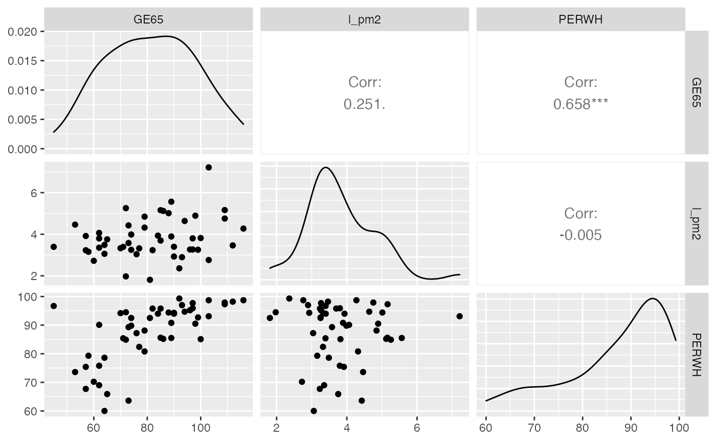

Modèle avec GE65, l_pm2 et NONPOOR

NONPOOR <- air_pollution$NONPOOR
predicteurs_sel <- data.frame(GE65,l_pm2,NONPOOR)
GGally::ggpairs(predicteurs_sel)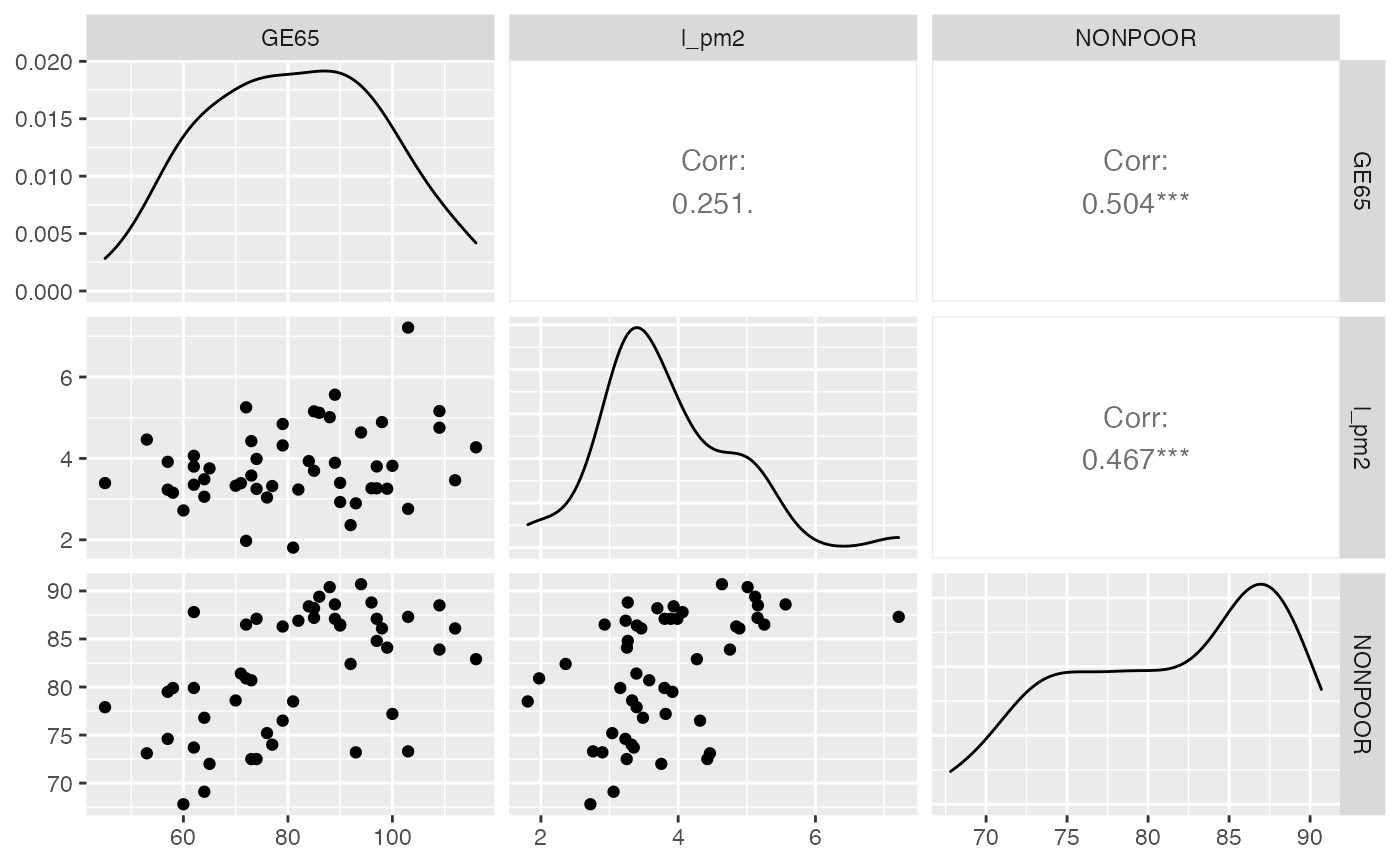

Description des données : Consommation d’électricité

Consommation d’électricité journalière en France de l’année 2003

Date : date
conso : consommation d’électricité en MWH
t : numéro du jour
nom_jour : nom du jour de la semaine
mois : nom du mois
temp : température en degrés Celsius
ejp : statut du jour EDF (spécial = 1 ; non spécial = 0)
ferie : statut du jour annuel (férié ou non)

Lecture des données

data(conso_temp)

Exercice 10.12 : Analyse descriptive

plot(conso_temp$temp, conso_temp$conso, xlab="Température",ylab="Consommation d'électricité")

plot(conso_temp$t, conso_temp$conso, type="l",xlab="Temps",ylab="Consommation d'électricité")

Exercice 10.13 : Plusieurs petits modèles

res.lm_conso_temp <- lm('conso~temp',data=conso_temp)
summary(res.lm_conso_temp)
#> 
#> Call:
#> lm(formula = "conso~temp", data = conso_temp)
#> 
#> Residuals:
#>     Min      1Q  Median      3Q     Max 
#> -692370 -148563   14133  181002  457884 
#> 
#> Coefficients:
#>             Estimate Std. Error t value Pr(>|t|)    
#> (Intercept)  3096889      25829  119.90   <2e-16 ***
#> temp          -46896       1741  -26.93   <2e-16 ***
#> ---
#> Signif. codes:  0 '***' 0.001 '**' 0.01 '*' 0.05 '.' 0.1 ' ' 1
#> 
#> Residual standard error: 238800 on 363 degrees of freedom
#> Multiple R-squared:  0.6665, Adjusted R-squared:  0.6656 
#> F-statistic: 725.4 on 1 and 363 DF,  p-value: < 2.2e-16

res.lm_conso_nom_jour <- lm('conso~nom_jour',data=conso_temp)
summary(res.lm_conso_nom_jour)
#> 
#> Call:
#> lm(formula = "conso~nom_jour", data = conso_temp)
#> 
#> Residuals:
#>     Min      1Q  Median      3Q     Max 
#> -770678 -288794 -170887  334431 1004436 
#> 
#> Coefficients:
#>                  Estimate Std. Error t value Pr(>|t|)    
#> (Intercept)       2165591      53080  40.799  < 2e-16 ***
#> nom_jourJeudi      429619      75066   5.723 2.21e-08 ***
#> nom_jourLundi      359886      75066   4.794 2.40e-06 ***
#> nom_jourMardi      442490      75066   5.895 8.68e-09 ***
#> nom_jourMercredi   454991      74711   6.090 2.91e-09 ***
#> nom_jourSamedi     155504      75066   2.072    0.039 *  
#> nom_jourVendredi   412957      75066   5.501 7.19e-08 ***
#> ---
#> Signif. codes:  0 '***' 0.001 '**' 0.01 '*' 0.05 '.' 0.1 ' ' 1
#> 
#> Residual standard error: 382800 on 358 degrees of freedom
#> Multiple R-squared:  0.1552, Adjusted R-squared:  0.141 
#> F-statistic: 10.96 on 6 and 358 DF,  p-value: 3.257e-11

res.lm_conso_mois <- lm('conso~mois',data=conso_temp)
summary(res.lm_conso_mois)
#> 
#> Call:
#> lm(formula = "conso~mois", data = conso_temp)
#> 
#> Residuals:
#>     Min      1Q  Median      3Q     Max 
#> -903710 -171027   46853  158783  511053 
#> 
#> Coefficients:
#>               Estimate Std. Error t value Pr(>|t|)    
#> (Intercept)    2032302      42394  47.938  < 2e-16 ***
#> moisAvril       392288      60452   6.489 2.92e-10 ***
#> moisDécembre    963815      59954  16.076  < 2e-16 ***
#> moisFévrier     954286      61539  15.507  < 2e-16 ***
#> moisJanvier     955814      59954  15.942  < 2e-16 ***
#> moisJuillet     183273      59954   3.057  0.00241 ** 
#> moisJuin        153228      60452   2.535  0.01169 *  
#> moisMai         111377      59954   1.858  0.06404 .  
#> moisMars        420908      59954   7.020 1.14e-11 ***
#> moisNovembre    701163      60452  11.599  < 2e-16 ***
#> moisOctobre     502472      59954   8.381 1.26e-15 ***
#> moisSeptembre   166700      60452   2.758  0.00613 ** 
#> ---
#> Signif. codes:  0 '***' 0.001 '**' 0.01 '*' 0.05 '.' 0.1 ' ' 1
#> 
#> Residual standard error: 236000 on 353 degrees of freedom
#> Multiple R-squared:  0.6832, Adjusted R-squared:  0.6733 
#> F-statistic: 69.21 on 11 and 353 DF,  p-value: < 2.2e-16

res.lm_conso_ejp <- lm('conso~ejp',data=conso_temp)
summary(res.lm_conso_ejp)
#> 
#> Call:
#> lm(formula = "conso~ejp", data = conso_temp)
#> 
#> Residuals:
#>     Min      1Q  Median      3Q     Max 
#> -728827 -234856  -73797  274354  947544 
#> 
#> Coefficients:
#>             Estimate Std. Error t value Pr(>|t|)    
#> (Intercept)  2441670      20398 119.701   <2e-16 ***
#> ejp           678776      77941   8.709   <2e-16 ***
#> ---
#> Signif. codes:  0 '***' 0.001 '**' 0.01 '*' 0.05 '.' 0.1 ' ' 1
#> 
#> Residual standard error: 376100 on 363 degrees of freedom
#> Multiple R-squared:  0.1728, Adjusted R-squared:  0.1705 
#> F-statistic: 75.84 on 1 and 363 DF,  p-value: < 2.2e-16

res.lm_conso_ferie <- lm('conso~ferie',data=conso_temp)
summary(res.lm_conso_ferie)
#> 
#> Call:
#> lm(formula = "conso~ferie", data = conso_temp)
#> 
#> Residuals:
#>     Min      1Q  Median      3Q     Max 
#> -788625 -257112 -113856  321808  970137 
#> 
#> Coefficients:
#>             Estimate Std. Error t value Pr(>|t|)    
#> (Intercept)  2501468      21609 115.762  < 2e-16 ***
#> ferieoui     -441526     124474  -3.547 0.000441 ***
#> ---
#> Signif. codes:  0 '***' 0.001 '**' 0.01 '*' 0.05 '.' 0.1 ' ' 1
#> 
#> Residual standard error: 406600 on 363 degrees of freedom
#> Multiple R-squared:  0.0335, Adjusted R-squared:  0.03084 
#> F-statistic: 12.58 on 1 and 363 DF,  p-value: 0.0004405

Exercice 10.14 : Modèle complet

Modèle complet

res.lm_conso_all <- lm('conso~temp+nom_jour+mois+ejp+ferie',data=conso_temp)
summary(res.lm_conso_all)
#> 
#> Call:
#> lm(formula = "conso~temp+nom_jour+mois+ejp+ferie", data = conso_temp)
#> 
#> Residuals:
#>     Min      1Q  Median      3Q     Max 
#> -451348  -63336    -503   65596  277071 
#> 
#> Coefficients:
#>                  Estimate Std. Error t value Pr(>|t|)    
#> (Intercept)       2598970      55304  46.994  < 2e-16 ***
#> temp               -36387       2108 -17.260  < 2e-16 ***
#> nom_jourJeudi      448914      21979  20.425  < 2e-16 ***
#> nom_jourLundi      375634      22036  17.047  < 2e-16 ***
#> nom_jourMardi      434728      21831  19.913  < 2e-16 ***
#> nom_jourMercredi   436470      21719  20.096  < 2e-16 ***
#> nom_jourSamedi     162655      21710   7.492 5.77e-13 ***
#> nom_jourVendredi   407251      22009  18.504  < 2e-16 ***
#> moisAvril          -56350      37699  -1.495 0.135906    
#> moisDécembre       287132      46564   6.166 1.96e-09 ***
#> moisFévrier        206940      49032   4.221 3.12e-05 ***
#> moisJanvier        192104      49439   3.886 0.000122 ***
#> moisJuillet         74649      28546   2.615 0.009315 ** 
#> moisJuin            66417      28755   2.310 0.021493 *  
#> moisMai           -182620      33408  -5.466 8.84e-08 ***
#> moisMars           -90910      39555  -2.298 0.022143 *  
#> moisNovembre       196805      41513   4.741 3.12e-06 ***
#> moisOctobre         -2434      39040  -0.062 0.950330    
#> moisSeptembre     -105467      31583  -3.339 0.000932 ***
#> ejp                 37347      27235   1.371 0.171173    
#> ferieoui          -426169      34816 -12.241  < 2e-16 ***
#> ---
#> Signif. codes:  0 '***' 0.001 '**' 0.01 '*' 0.05 '.' 0.1 ' ' 1
#> 
#> Residual standard error: 110600 on 344 degrees of freedom
#> Multiple R-squared:  0.9322, Adjusted R-squared:  0.9283 
#> F-statistic: 236.5 on 20 and 344 DF,  p-value: < 2.2e-16
SCT <- sum((conso_temp$conso-mean(conso_temp$conso))^2)
resid <- res.lm_conso_all$residuals
SCR_all <- 364*var(resid)
SCE_all <- SCT-SCR_all

Calcul de l’apport de chaque variable du modèle à l’aide du \(F\) partiel

variable <- matrix(0,nrow=5)
f_partiel <- matrix(0,nrow=5)
p_value <- matrix(0,nrow=5)
nu_1 <- matrix(0,nrow=5)
nu_2 <- matrix(0,nrow=5)

Modèle sans temp

res.lm_conso_all_temp <- lm('conso~nom_jour+mois+ejp+ferie',data=conso_temp)
summary(res.lm_conso_all_temp)
#> 
#> Call:
#> lm(formula = "conso~nom_jour+mois+ejp+ferie", data = conso_temp)
#> 
#> Residuals:
#>     Min      1Q  Median      3Q     Max 
#> -702695  -86287    7982   64969  549209 
#> 
#> Coefficients:
#>                  Estimate Std. Error t value Pr(>|t|)    
#> (Intercept)       1741637      33169  52.508  < 2e-16 ***
#> nom_jourJeudi      445230      29979  14.852  < 2e-16 ***
#> nom_jourLundi      360841      30035  12.014  < 2e-16 ***
#> nom_jourMardi      432122      29778  14.512  < 2e-16 ***
#> nom_jourMercredi   429988      29621  14.516  < 2e-16 ***
#> nom_jourSamedi     164855      29613   5.567 5.21e-08 ***
#> nom_jourVendredi   395312      30006  13.174  < 2e-16 ***
#> moisAvril          372535      38672   9.633  < 2e-16 ***
#> moisDécembre       926320      38502  24.059  < 2e-16 ***
#> moisFévrier        879036      40644  21.628  < 2e-16 ***
#> moisJanvier        879180      39993  21.983  < 2e-16 ***
#> moisJuillet        159171      38361   4.149 4.20e-05 ***
#> moisJuin           150183      38660   3.885 0.000123 ***
#> moisMai            126884      38449   3.300 0.001068 ** 
#> moisMars           385598      38639   9.979  < 2e-16 ***
#> moisNovembre       720084      38682  18.615  < 2e-16 ***
#> moisOctobre        464623      38385  12.104  < 2e-16 ***
#> moisSeptembre      133819      38708   3.457 0.000614 ***
#> ejp                166527      35719   4.662 4.48e-06 ***
#> ferieoui          -462962      47401  -9.767  < 2e-16 ***
#> ---
#> Signif. codes:  0 '***' 0.001 '**' 0.01 '*' 0.05 '.' 0.1 ' ' 1
#> 
#> Residual standard error: 150900 on 345 degrees of freedom
#> Multiple R-squared:  0.8735, Adjusted R-squared:  0.8665 
#> F-statistic: 125.4 on 19 and 345 DF,  p-value: < 2.2e-16
resid <- res.lm_conso_all_temp$residuals
SCR_temp <-364*var(resid)
SCE_temp <- SCT-SCR_temp
f_temp=((SCE_all-SCE_temp)/(1))/(SCR_all/344)
p_val_temp = 1-pf(f_temp,1,344)
variable[1] <- "temp"
f_partiel[1] <- f_temp
p_value[1] <- p_val_temp
nu_1[1] <- 1
nu_2[1] <- 344

Modèle sans nom_jour

res.lm_conso_all_nom_jour <- lm('conso~temp+mois+ejp+ferie',data=conso_temp)
summary(res.lm_conso_all_nom_jour)
#> 
#> Call:
#> lm(formula = "conso~temp+mois+ejp+ferie", data = conso_temp)
#> 
#> Residuals:
#>     Min      1Q  Median      3Q     Max 
#> -630398 -113728   35907  142429  363782 
#> 
#> Coefficients:
#>               Estimate Std. Error t value Pr(>|t|)    
#> (Intercept)    2865800      94502  30.325  < 2e-16 ***
#> temp            -34648       3704  -9.355  < 2e-16 ***
#> moisAvril       -15554      66250  -0.235  0.81452    
#> moisDécembre    327835      81827   4.006 7.53e-05 ***
#> moisFévrier     220265      86242   2.554  0.01107 *  
#> moisJanvier     209386      86960   2.408  0.01656 *  
#> moisJuillet     102883      50178   2.050  0.04107 *  
#> moisJuin         74196      50566   1.467  0.14319    
#> moisMai        -158730      58752  -2.702  0.00723 ** 
#> moisMars        -82017      69554  -1.179  0.23912    
#> moisNovembre    215735      73000   2.955  0.00334 ** 
#> moisOctobre      45864      68580   0.669  0.50408    
#> moisSeptembre   -72995      55491  -1.315  0.18923    
#> ejp             163930      46797   3.503  0.00052 ***
#> ferieoui       -344641      60567  -5.690 2.68e-08 ***
#> ---
#> Signif. codes:  0 '***' 0.001 '**' 0.01 '*' 0.05 '.' 0.1 ' ' 1
#> 
#> Residual standard error: 194600 on 350 degrees of freedom
#> Multiple R-squared:  0.7864, Adjusted R-squared:  0.7779 
#> F-statistic: 92.06 on 14 and 350 DF,  p-value: < 2.2e-16
resid <- res.lm_conso_all_nom_jour$residuals
SCR_nom_jour <-364*var(resid)
SCE_nom_jour <- SCT-SCR_nom_jour
f_nom_jour=((SCE_all-SCE_nom_jour)/(6))/(SCR_all/344)
p_val_nom_jour = 1-pf(f_nom_jour,6,344)
variable[2] <- "nom_jour"
f_partiel[2] <- f_nom_jour
p_value[2] <- p_val_nom_jour
nu_1[2] <- 6
nu_2[2] <- 344

Modèle sans mois

res.lm_conso_all_mois <- lm('conso~temp+nom_jour+ejp+ferie',data=conso_temp)
summary(res.lm_conso_all_mois)
#> 
#> Call:
#> lm(formula = "conso~temp+nom_jour+ejp+ferie", data = conso_temp)
#> 
#> Residuals:
#>     Min      1Q  Median      3Q     Max 
#> -409421 -130397   -2182  132234  366626 
#> 
#> Coefficients:
#>                  Estimate Std. Error t value Pr(>|t|)    
#> (Intercept)       2762583      29064  95.052  < 2e-16 ***
#> temp               -45087       1327 -33.970  < 2e-16 ***
#> nom_jourJeudi      441220      33115  13.324  < 2e-16 ***
#> nom_jourLundi      370313      33180  11.161  < 2e-16 ***
#> nom_jourMardi      429878      32877  13.076  < 2e-16 ***
#> nom_jourMercredi   434874      32713  13.293  < 2e-16 ***
#> nom_jourSamedi     156265      32753   4.771 2.68e-06 ***
#> nom_jourVendredi   397181      33141  11.984  < 2e-16 ***
#> ejp                 65601      38437   1.707   0.0888 .  
#> ferieoui          -415458      51776  -8.024 1.51e-14 ***
#> ---
#> Signif. codes:  0 '***' 0.001 '**' 0.01 '*' 0.05 '.' 0.1 ' ' 1
#> 
#> Residual standard error: 166900 on 355 degrees of freedom
#> Multiple R-squared:  0.8407, Adjusted R-squared:  0.8366 
#> F-statistic: 208.1 on 9 and 355 DF,  p-value: < 2.2e-16
resid <- res.lm_conso_all_mois$residuals
SCR_mois <-364*var(resid)
SCE_mois <- SCT-SCR_mois
f_mois=((SCE_all-SCE_mois)/(11))/(SCR_all/344)
p_val_mois = 1-pf(f_mois,11,344)
variable[3] <- "mois"
f_partiel[3] <- f_mois
p_value[3] <- p_val_mois
nu_1[3] <- 11
nu_2[3] <- 344

Modèle sans ejp

res.lm_conso_all_ejp <- lm('conso~temp+nom_jour+mois+ferie',data=conso_temp)
summary(res.lm_conso_all_ejp)
#> 
#> Call:
#> lm(formula = "conso~temp+nom_jour+mois+ferie", data = conso_temp)
#> 
#> Residuals:
#>     Min      1Q  Median      3Q     Max 
#> -457304  -63748    -802   65726  268560 
#> 
#> Coefficients:
#>                  Estimate Std. Error t value Pr(>|t|)    
#> (Intercept)       2615465      54049  48.391  < 2e-16 ***
#> temp               -37181       2030 -18.320  < 2e-16 ***
#> nom_jourJeudi      451690      21913  20.613  < 2e-16 ***
#> nom_jourLundi      380006      21832  17.406  < 2e-16 ***
#> nom_jourMardi      437513      21764  20.103  < 2e-16 ***
#> nom_jourMercredi   439124      21660  20.274  < 2e-16 ***
#> nom_jourSamedi     162645      21738   7.482 6.13e-13 ***
#> nom_jourVendredi   412078      21753  18.943  < 2e-16 ***
#> moisAvril          -65809      37110  -1.773 0.077054 .  
#> moisDécembre       276367      45956   6.014 4.62e-09 ***
#> moisFévrier        201983      48961   4.125 4.64e-05 ***
#> moisJanvier        188074      49415   3.806 0.000167 ***
#> moisJuillet         72696      28547   2.547 0.011313 *  
#> moisJuin            64533      28759   2.244 0.025470 *  
#> moisMai           -189332      33090  -5.722 2.29e-08 ***
#> moisMars           -96908      39362  -2.462 0.014307 *  
#> moisNovembre       185527      40742   4.554 7.32e-06 ***
#> moisOctobre        -12864      38341  -0.336 0.737432    
#> moisSeptembre     -110907      31373  -3.535 0.000463 ***
#> ferieoui          -427425      34848 -12.265  < 2e-16 ***
#> ---
#> Signif. codes:  0 '***' 0.001 '**' 0.01 '*' 0.05 '.' 0.1 ' ' 1
#> 
#> Residual standard error: 110800 on 345 degrees of freedom
#> Multiple R-squared:  0.9318, Adjusted R-squared:  0.9281 
#> F-statistic: 248.2 on 19 and 345 DF,  p-value: < 2.2e-16
resid <- res.lm_conso_all_ejp$residuals
SCR_ejp <-364*var(resid)
SCE_ejp <- SCT-SCR_ejp
f_ejp=((SCE_all-SCE_ejp)/(1))/(SCR_all/344)
p_val_ejp = 1-pf(f_ejp,1,344)
variable[4] <- "ejp"
f_partiel[4] <- f_ejp
p_value[4] <- p_val_ejp
nu_1[4] <- 1
nu_2[4] <- 344

Modèle sans ferie

res.lm_conso_all_ferie <- lm('conso~temp+nom_jour+mois+ejp',data=conso_temp)
summary(res.lm_conso_all_ferie)
#> 
#> Call:
#> lm(formula = "conso~temp+nom_jour+mois+ejp", data = conso_temp)
#> 
#> Residuals:
#>     Min      1Q  Median      3Q     Max 
#> -772831  -64226    8971   76576  270685 
#> 
#> Coefficients:
#>                  Estimate Std. Error t value Pr(>|t|)    
#> (Intercept)       2635541      66070  39.890  < 2e-16 ***
#> temp               -37967       2518 -15.081  < 2e-16 ***
#> nom_jourJeudi      415540      26093  15.926  < 2e-16 ***
#> nom_jourLundi      349569      26240  13.322  < 2e-16 ***
#> nom_jourMardi      425238      26102  16.291  < 2e-16 ***
#> nom_jourMercredi   427407      25969  16.458  < 2e-16 ***
#> nom_jourSamedi     154906      25963   5.966 6.01e-09 ***
#> nom_jourVendredi   397921      26316  15.121  < 2e-16 ***
#> moisAvril          -74946      45067  -1.663  0.09722 .  
#> moisDécembre       258894      55641   4.653 4.67e-06 ***
#> moisFévrier        188116      58633   3.208  0.00146 ** 
#> moisJanvier        158767      59060   2.688  0.00753 ** 
#> moisJuillet         72107      34152   2.111  0.03546 *  
#> moisJuin            63065      34401   1.833  0.06763 .  
#> moisMai           -222369      39780  -5.590 4.62e-08 ***
#> moisMars           -99217      47317  -2.097  0.03673 *  
#> moisNovembre       159581      49533   3.222  0.00140 ** 
#> moisOctobre         -7882      46705  -0.169  0.86609    
#> moisSeptembre     -101100      37784  -2.676  0.00781 ** 
#> ejp                 46121      32573   1.416  0.15770    
#> ---
#> Signif. codes:  0 '***' 0.001 '**' 0.01 '*' 0.05 '.' 0.1 ' ' 1
#> 
#> Residual standard error: 132300 on 345 degrees of freedom
#> Multiple R-squared:  0.9027, Adjusted R-squared:  0.8973 
#> F-statistic: 168.4 on 19 and 345 DF,  p-value: < 2.2e-16
resid <- res.lm_conso_all_ferie$residuals
SCR_ferie <-364*var(resid)
SCE_ferie <- SCT-SCR_ferie
f_ferie=((SCE_all-SCE_ferie)/(1))/(SCR_all/344)
p_val_ferie = 1-pf(f_ferie,1,344)
variable[5] <- "ferie"
f_partiel[5] <- f_ferie
p_value[5] <- p_val_ferie
nu_1[5] <- 1
nu_2[5] <- 344

f_partiel <- round(f_partiel,2)
p_value <- round(p_value,4)

tab_result <- data.frame(variable,f_partiel,nu_1,nu_2,p_value)

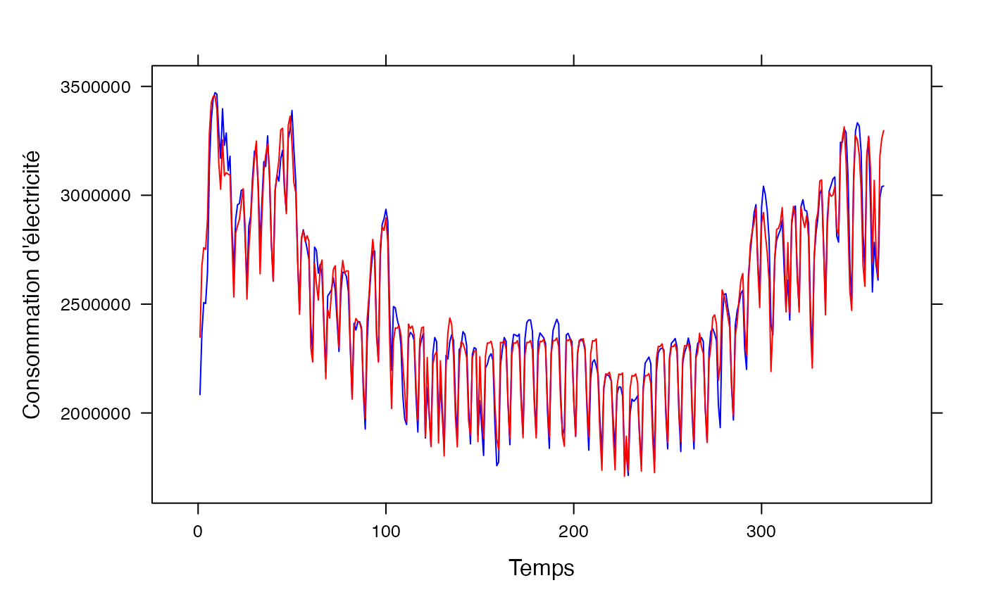
pred <- predict(res.lm_conso_all)
lattice::xyplot(conso_temp$conso+pred~conso_temp$t,type="l",xlab="Temps",ylab="Consommation d'électricité",col=c("blue","red"))

Exercice 10.15 : Un modèle « à la main »

pred <- predict(res.lm_conso_all_ejp)
lattice::xyplot(conso_temp$conso+pred~conso_temp$t,type="l",xlab="Temps",ylab="Consommation d'électricité",col=c("blue","red"))

Exercice 10.16 : Amélioration du modèle

Création de la variable catégorielle pour la variable température

temp_cat <- matrix(0,nrow=365)
for (i in 1:365)
    {if (conso_temp$temp[i] < 15) {temp_cat[i]="< 15°C"}
        else {temp_cat[i]=">= 15°C"}
    }
conso_temp <- data.frame(conso_temp,temp_cat)

Modèle avec interaction

res.lm_conso_interaction <- lm('conso~temp_cat+temp_cat:temp+nom_jour+mois+ferie',data=conso_temp)
summary(res.lm_conso_interaction)
#> 
#> Call:
#> lm(formula = "conso~temp_cat+temp_cat:temp+nom_jour+mois+ferie", 
#>     data = conso_temp)
#> 
#> Residuals:
#>     Min      1Q  Median      3Q     Max 
#> -310536  -44343    5330   50004  219595 
#> 
#> Coefficients:
#>                      Estimate Std. Error t value Pr(>|t|)    
#> (Intercept)           2507322      42119  59.529  < 2e-16 ***
#> temp_cat>= 15°C       -801107      62550 -12.807  < 2e-16 ***
#> nom_jourJeudi          449495      16904  26.592  < 2e-16 ***
#> nom_jourLundi          381074      16782  22.708  < 2e-16 ***
#> nom_jourMardi          440276      16724  26.325  < 2e-16 ***
#> nom_jourMercredi       438833      16657  26.345  < 2e-16 ***
#> nom_jourSamedi         161271      16713   9.650  < 2e-16 ***
#> nom_jourVendredi       407964      16749  24.357  < 2e-16 ***
#> moisAvril              225840      34140   6.615 1.43e-10 ***
#> moisDécembre           491569      38135  12.890  < 2e-16 ***
#> moisFévrier            387779      39608   9.790  < 2e-16 ***
#> moisJanvier            364928      39757   9.179  < 2e-16 ***
#> moisJuillet            161472      22902   7.050 9.87e-12 ***
#> moisJuin               152211      23042   6.606 1.51e-10 ***
#> moisMai                118947      32258   3.687 0.000263 ***
#> moisMars               197024      36149   5.450 9.63e-08 ***
#> moisNovembre           465714      36539  12.746  < 2e-16 ***
#> moisOctobre            273485      34966   7.821 6.51e-14 ***
#> moisSeptembre          140706      29777   4.725 3.36e-06 ***
#> ferieoui              -430840      26782 -16.087  < 2e-16 ***
#> temp_cat< 15°C:temp    -55429       2003 -27.679  < 2e-16 ***
#> temp_cat>= 15°C:temp     1162       3254   0.357 0.721318    
#> ---
#> Signif. codes:  0 '***' 0.001 '**' 0.01 '*' 0.05 '.' 0.1 ' ' 1
#> 
#> Residual standard error: 85100 on 343 degrees of freedom
#> Multiple R-squared:   0.96,  Adjusted R-squared:  0.9575 
#> F-statistic: 391.8 on 21 and 343 DF,  p-value: < 2.2e-16
SCT <- sum((conso_temp$conso-mean(conso_temp$conso))^2)
resid <- res.lm_conso_interaction$residuals
SCR_interaction <- 364*var(resid)
SCE_interaction <- SCT-SCR_interaction

Modèle sans interaction

res.lm_conso_sans_inter <- lm('conso~temp+nom_jour+mois+ferie',data=conso_temp)
summary(res.lm_conso_sans_inter)
#> 
#> Call:
#> lm(formula = "conso~temp+nom_jour+mois+ferie", data = conso_temp)
#> 
#> Residuals:
#>     Min      1Q  Median      3Q     Max 
#> -457304  -63748    -802   65726  268560 
#> 
#> Coefficients:
#>                  Estimate Std. Error t value Pr(>|t|)    
#> (Intercept)       2615465      54049  48.391  < 2e-16 ***
#> temp               -37181       2030 -18.320  < 2e-16 ***
#> nom_jourJeudi      451690      21913  20.613  < 2e-16 ***
#> nom_jourLundi      380006      21832  17.406  < 2e-16 ***
#> nom_jourMardi      437513      21764  20.103  < 2e-16 ***
#> nom_jourMercredi   439124      21660  20.274  < 2e-16 ***
#> nom_jourSamedi     162645      21738   7.482 6.13e-13 ***
#> nom_jourVendredi   412078      21753  18.943  < 2e-16 ***
#> moisAvril          -65809      37110  -1.773 0.077054 .  
#> moisDécembre       276367      45956   6.014 4.62e-09 ***
#> moisFévrier        201983      48961   4.125 4.64e-05 ***
#> moisJanvier        188074      49415   3.806 0.000167 ***
#> moisJuillet         72696      28547   2.547 0.011313 *  
#> moisJuin            64533      28759   2.244 0.025470 *  
#> moisMai           -189332      33090  -5.722 2.29e-08 ***
#> moisMars           -96908      39362  -2.462 0.014307 *  
#> moisNovembre       185527      40742   4.554 7.32e-06 ***
#> moisOctobre        -12864      38341  -0.336 0.737432    
#> moisSeptembre     -110907      31373  -3.535 0.000463 ***
#> ferieoui          -427425      34848 -12.265  < 2e-16 ***
#> ---
#> Signif. codes:  0 '***' 0.001 '**' 0.01 '*' 0.05 '.' 0.1 ' ' 1
#> 
#> Residual standard error: 110800 on 345 degrees of freedom
#> Multiple R-squared:  0.9318, Adjusted R-squared:  0.9281 
#> F-statistic: 248.2 on 19 and 345 DF,  p-value: < 2.2e-16
resid <- res.lm_conso_sans_inter$residuals
SCR_sans_inter <- 364*var(resid)
SCE_sans_inter <- SCT-SCR_sans_inter
f_inter=((SCE_interaction-SCE_sans_inter)/(2))/(SCR_interaction/344)
p_val_inter = 1-pf(f_inter,2,344)
variable <- "interaction"
f_partiel <- f_inter
p_value <- p_val_inter
nu_1 <- 2
nu_2 <- 344

tab_result <- data.frame(variable,f_partiel,nu_1,nu_2,p_value)

pred <- predict(res.lm_conso_interaction)
lattice::xyplot(conso_temp$conso+pred~conso_temp$t,type="l",xlab="Temps",ylab="Consommation d'électricité",col=c("blue","red"))

Tout le code avec R.

Christian Derquenne

2022-09-21