Chapitre 09. Inférence statistique.

if(!("sageR" %in% installed.packages())){install.packages("sageR")}
library(sageR)

Intervalles de confiance

Pour la moyenne

data(Flux)
mean(Flux)
#> [1] 13.99533

shapiro.test(Flux)
#> 
#>  Shapiro-Wilk normality test
#> 
#> data:  Flux
#> W = 0.97931, p-value = 0.8068

qqnorm(Flux)
qqline(Flux)

t.test(Flux)
#> 
#>  One Sample t-test
#> 
#> data:  Flux
#> t = 80.878, df = 29, p-value < 2.2e-16
#> alternative hypothesis: true mean is not equal to 0
#> 95 percent confidence interval:
#>  13.64142 14.34925
#> sample estimates:
#> mean of x 
#>  13.99533

Pour la variance

var(Flux)
#> [1] 0.8983154

L’hypothèse de normalité a déjà été validée au seuil $\alpha=5\%$

if(!("TeachingDemos" %in% installed.packages())){install.packages("TeachingDemos")}
library(TeachingDemos)
TeachingDemos::sigma.test(Flux)
#> 
#>  One sample Chi-squared test for variance
#> 
#> data:  Flux
#> X-squared = 26.051, df = 29, p-value = 0.7545
#> alternative hypothesis: true variance is not equal to 1
#> 95 percent confidence interval:
#>  0.5697691 1.6234206
#> sample estimates:
#> var of Flux 
#>   0.8983154

Test $t$ pour un échantillon

data(Precipitations_USA)
colnames(Precipitations_USA) <- c("Ville", "Precipitation (inches)", "Precipitation (cms)", "Etat")
if(!("ggmap" %in% installed.packages())){install.packages("ggmap")}
library(ggmap)
#> Loading required package: ggplot2
#> ℹ Google's Terms of Service: <https://mapsplatform.google.com>
#>   Stadia Maps' Terms of Service: <https://stadiamaps.com/terms-of-service>
#>   OpenStreetMap's Tile Usage Policy: <https://operations.osmfoundation.org/policies/tiles>
#> ℹ Please cite ggmap if you use it! Use `citation("ggmap")` for details.
if(!("tidygeocoder" %in% installed.packages())){install.packages("tidygeocoder")}
library(tidygeocoder)
#> 
#> Attaching package: 'tidygeocoder'
#> 
#> The following object is masked from 'package:ggmap':
#> 
#>     geocode
levels(Precipitations_USA[,1]) <- gsub("Philadelphie","Philadelphia",levels(Precipitations_USA[,1]))
levels(Precipitations_USA[,1]) <- gsub("Washington. D.C.","Washington",levels(Precipitations_USA[,1]))
gps_coords <- mapply(tidygeocoder::geo, city= Precipitations_USA[,1], state = Precipitations_USA[,4], method = "osm")
#> Passing 1 address to the Nominatim single address geocoder
#> Query completed in: 1 seconds
#> Passing 1 address to the Nominatim single address geocoder
#> Query completed in: 1 seconds
#> Passing 1 address to the Nominatim single address geocoder
#> Query completed in: 1 seconds
#> Passing 1 address to the Nominatim single address geocoder
#> Query completed in: 1 seconds
#> Passing 1 address to the Nominatim single address geocoder
#> Query completed in: 1 seconds
#> Passing 1 address to the Nominatim single address geocoder
#> Query completed in: 1 seconds
#> Passing 1 address to the Nominatim single address geocoder
#> Query completed in: 1 seconds
#> Passing 1 address to the Nominatim single address geocoder
#> Query completed in: 1 seconds
#> Passing 1 address to the Nominatim single address geocoder
#> Query completed in: 1 seconds
#> Passing 1 address to the Nominatim single address geocoder
#> Query completed in: 1 seconds
#> Passing 1 address to the Nominatim single address geocoder
#> Query completed in: 1 seconds
#> Passing 1 address to the Nominatim single address geocoder
#> Query completed in: 1 seconds
#> Passing 1 address to the Nominatim single address geocoder
#> Query completed in: 1 seconds
#> Passing 1 address to the Nominatim single address geocoder
#> Query completed in: 1 seconds
#> Passing 1 address to the Nominatim single address geocoder
#> Query completed in: 1 seconds
#> Passing 1 address to the Nominatim single address geocoder
#> Query completed in: 1 seconds
#> Passing 1 address to the Nominatim single address geocoder
#> Query completed in: 1 seconds
#> Passing 1 address to the Nominatim single address geocoder
#> Query completed in: 1 seconds
#> Passing 1 address to the Nominatim single address geocoder
#> Query completed in: 1 seconds
#> Passing 1 address to the Nominatim single address geocoder
#> Query completed in: 1 seconds
#> Passing 1 address to the Nominatim single address geocoder
#> Query completed in: 1 seconds
#> Passing 1 address to the Nominatim single address geocoder
#> Query completed in: 1 seconds
#> Passing 1 address to the Nominatim single address geocoder
#> Query completed in: 1 seconds
#> Passing 1 address to the Nominatim single address geocoder
#> Query completed in: 1 seconds
#> Passing 1 address to the Nominatim single address geocoder
#> Query completed in: 1 seconds
#> Passing 1 address to the Nominatim single address geocoder
#> Query completed in: 1 seconds
#> Passing 1 address to the Nominatim single address geocoder
#> Query completed in: 1 seconds
#> Passing 1 address to the Nominatim single address geocoder
#> Query completed in: 1 seconds
#> Passing 1 address to the Nominatim single address geocoder
#> Query completed in: 1 seconds
#> Passing 1 address to the Nominatim single address geocoder
#> Query completed in: 1 seconds
#> Passing 1 address to the Nominatim single address geocoder
#> Query completed in: 1 seconds
#> Passing 1 address to the Nominatim single address geocoder
#> Query completed in: 1 seconds
#> Passing 1 address to the Nominatim single address geocoder
#> Query completed in: 1 seconds
#> Passing 1 address to the Nominatim single address geocoder
#> Query completed in: 1 seconds
#> Passing 1 address to the Nominatim single address geocoder
#> Query completed in: 1 seconds
#> Passing 1 address to the Nominatim single address geocoder
#> Query completed in: 1 seconds
#> Passing 1 address to the Nominatim single address geocoder
#> Query completed in: 1 seconds
#> Passing 1 address to the Nominatim single address geocoder
#> Query completed in: 1 seconds
#> Passing 1 address to the Nominatim single address geocoder
#> Query completed in: 1 seconds
#> Passing 1 address to the Nominatim single address geocoder
#> Query completed in: 1 seconds
#> Passing 1 address to the Nominatim single address geocoder
#> Query completed in: 1 seconds
#> Passing 1 address to the Nominatim single address geocoder
#> Query completed in: 1 seconds
#> Passing 1 address to the Nominatim single address geocoder
#> Query completed in: 1 seconds
#> Passing 1 address to the Nominatim single address geocoder
#> Query completed in: 1 seconds
#> Passing 1 address to the Nominatim single address geocoder
#> Query completed in: 1 seconds
#> Passing 1 address to the Nominatim single address geocoder
#> Query completed in: 1 seconds
#> Passing 1 address to the Nominatim single address geocoder
#> Query completed in: 1 seconds
#> Passing 1 address to the Nominatim single address geocoder
#> Query completed in: 1 seconds
#> Passing 1 address to the Nominatim single address geocoder
#> Query completed in: 1 seconds
#> Passing 1 address to the Nominatim single address geocoder
#> Query completed in: 1 seconds
#> Passing 1 address to the Nominatim single address geocoder
#> Query completed in: 1 seconds
#> Passing 1 address to the Nominatim single address geocoder
#> Query completed in: 1 seconds
#> Passing 1 address to the Nominatim single address geocoder
#> Query completed in: 1 seconds
#> Passing 1 address to the Nominatim single address geocoder
#> Query completed in: 1 seconds
#> Passing 1 address to the Nominatim single address geocoder
#> Query completed in: 1 seconds
#> Passing 1 address to the Nominatim single address geocoder
#> Query completed in: 1 seconds
#> Passing 1 address to the Nominatim single address geocoder
#> Query completed in: 1 seconds
#> Passing 1 address to the Nominatim single address geocoder
#> Query completed in: 1 seconds
#> Passing 1 address to the Nominatim single address geocoder
#> Query completed in: 1 seconds
#> Passing 1 address to the Nominatim single address geocoder
#> Query completed in: 1 seconds
levels(Precipitations_USA[,1]) <- gsub("Philadelphia","Philadelphie",levels(Precipitations_USA[,1]))
gps_coords[1,gps_coords[1,]=="Philadelphia"] <- "Philadelphie"
gps_coords[1,gps_coords[1,]=="Washington"] <- "Washington. D.C."

gps_coords_df <- as.data.frame(matrix(unlist(gps_coords),ncol=4,byrow=TRUE))
colnames(gps_coords_df) <- c("Ville", "Etat", "lat", "long")
gps_coords_df$lat <- as.numeric(gps_coords_df$lat)
gps_coords_df$long <- as.numeric(gps_coords_df$long)

precip_gps <- merge(Precipitations_USA,gps_coords_df)

precip_gps_map <- ggmap::get_map(c(left = min(gps_coords_df$long)*1.03, bottom = min(gps_coords_df$lat)/1.2, right = max(gps_coords_df$long)/1.12, top = max(gps_coords_df$lat))*1.03, maptype="stamen_terrain", source = "stadia", zoom=5, messaging = FALSE)
#> ℹ © Stadia Maps © Stamen Design © OpenMapTiles © OpenStreetMap contributors.
#> ℹ 60 tiles needed, this may take a while (try a smaller zoom?)

ggmap::ggmap(precip_gps_map,extent = "device") + 
  geom_point(aes(x = long, y = lat, color=`Precipitation (cms)`),
             data = precip_gps, size = 5, pch = 20) + 
  scale_color_gradient(low="red", high="blue")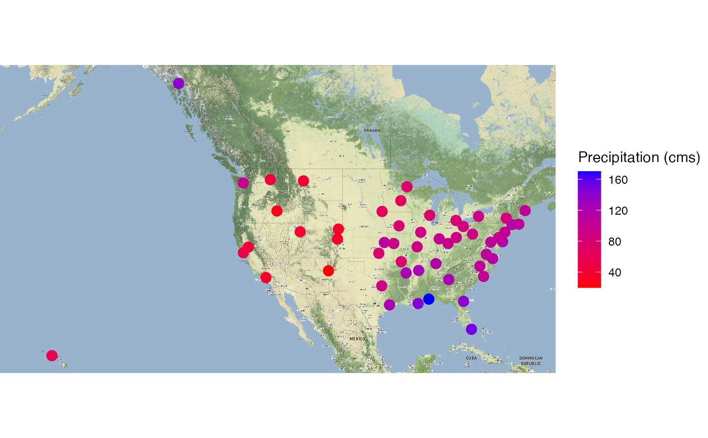

ggplot2::ggsave("map_pprecip_USA.pdf", width=14, height=8)

precip_gps_map_bw <- ggmap::get_stadiamap(c(left = min(gps_coords_df$long)*1.03, bottom = min(gps_coords_df$lat)/1.2, right = max(gps_coords_df$long)/1.12, top = max(gps_coords_df$lat))*1.03, source = "stamen", zoom=5, maptype="stamen_toner")
#> ℹ © Stadia Maps © Stamen Design © OpenMapTiles © OpenStreetMap contributors.
#> ℹ 60 tiles needed, this may take a while (try a smaller zoom?)

ggmap::ggmap(precip_gps_map_bw,extent = "device") + 
  geom_point(aes(x = long, y = lat, color=`Precipitation (cms)`),
             data = precip_gps, size = 5, pch = 20, fill = "white") + 
  scale_color_gradient(low="white", high="black")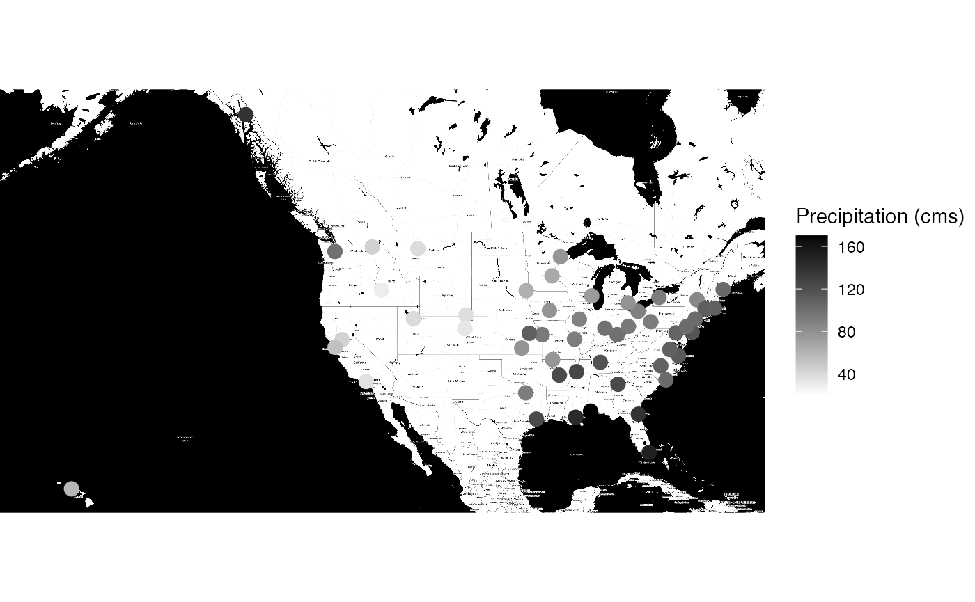

with(Precipitations_USA, shapiro.test(`Precipitation (cms)`))
#> 
#>  Shapiro-Wilk normality test
#> 
#> data:  Precipitation (cms)
#> W = 0.97241, p-value = 0.1911

with(Precipitations_USA,qqnorm(`Precipitation (cms)`))
with(Precipitations_USA,qqline(`Precipitation (cms)`))

with(Precipitations_USA, t.test(`Precipitation (cms)`, mu = 83.90))
#> 
#>  One Sample t-test
#> 
#> data:  Precipitation (cms)
#> t = 1.6898, df = 59, p-value = 0.09635
#> alternative hypothesis: true mean is not equal to 83.9
#> 95 percent confidence interval:
#>  82.61107 99.18519
#> sample estimates:
#> mean of x 
#>  90.89813

with(Precipitations_USA, TeachingDemos::sigma.test(`Precipitation (cms)`))
#> 
#>  One sample Chi-squared test for variance
#> 
#> data:  Precipitation (cms)
#> X-squared = 60717, df = 59, p-value < 2.2e-16
#> alternative hypothesis: true variance is not equal to 1
#> 95 percent confidence interval:
#>   739.3954 1530.8720
#> sample estimates:
#> var of Precipitation (cms) 
#>                   1029.106

ggplot2::ggsave("map_pprecip_USA_bw.pdf", width=14, height=8)

data(Resistance)

qqnorm(Resistance)
qqline(Resistance)

if(!("TeachingDemos" %in% installed.packages())){install.packages("TeachingDemos")}
TeachingDemos::sigma.test(Resistance,sigmasq = 8)
#> 
#>  One sample Chi-squared test for variance
#> 
#> data:  Resistance
#> X-squared = 38.47, df = 29, p-value = 0.2245
#> alternative hypothesis: true variance is not equal to 8
#> 95 percent confidence interval:
#>   6.731113 19.178694
#> sample estimates:
#> var of Resistance 
#>          10.61248

binom.test(30,200,p=0.10,alternative=c("greater"))
#> 
#>  Exact binomial test
#> 
#> data:  30 and 200
#> number of successes = 30, number of trials = 200, p-value = 0.01633
#> alternative hypothesis: true probability of success is greater than 0.1
#> 95 percent confidence interval:
#>  0.1100814 1.0000000
#> sample estimates:
#> probability of success 
#>                   0.15

Test $t$ pour deux échantillons indépendants.

data(Essence)

shapiro.test(Essence$Aube)
#> 
#>  Shapiro-Wilk normality test
#> 
#> data:  Essence$Aube
#> W = 0.97524, p-value = 0.6897

with(Essence,qqnorm(Aube))
with(Essence,qqline(Aube))

shapiro.test(Essence$Marne)
#> 
#>  Shapiro-Wilk normality test
#> 
#> data:  Essence$Marne
#> W = 0.95879, p-value = 0.2884

with(Essence,qqnorm(Marne))
with(Essence,qqline(Marne))

mean(Essence$Aube)
#> [1] 1.529867
mean(Essence$Marne)
#> [1] 1.4241

with(Essence, var.test(x=Aube,y=Marne))
#> 
#>  F test to compare two variances
#> 
#> data:  Aube and Marne
#> F = 1.6155, num df = 29, denom df = 29, p-value = 0.2025
#> alternative hypothesis: true ratio of variances is not equal to 1
#> 95 percent confidence interval:
#>  0.7689431 3.3942558
#> sample estimates:
#> ratio of variances 
#>           1.615546

with(Essence, t.test(x=Aube,y=Marne, var.equal = TRUE))
#> 
#>  Two Sample t-test
#> 
#> data:  Aube and Marne
#> t = 21.852, df = 58, p-value < 2.2e-16
#> alternative hypothesis: true difference in means is not equal to 0
#> 95 percent confidence interval:
#>  0.0960779 0.1154554
#> sample estimates:
#> mean of x mean of y 
#>  1.529867  1.424100

with(Essence, t.test(x=Aube,y=Marne))
#> 
#>  Welch Two Sample t-test
#> 
#> data:  Aube and Marne
#> t = 21.852, df = 54.956, p-value < 2.2e-16
#> alternative hypothesis: true difference in means is not equal to 0
#> 95 percent confidence interval:
#>  0.09606647 0.11546687
#> sample estimates:
#> mean of x mean of y 
#>  1.529867  1.424100

Test $t$ pour deux échantillons appariés

with(Copies,shapiro.test(Correcteur.A-Correcteur.B))
#> 
#>  Shapiro-Wilk normality test
#> 
#> data:  Correcteur.A - Correcteur.B
#> W = 0.97738, p-value = 0.7524

with(Copies,qqnorm(Correcteur.A-Correcteur.B))
with(Copies,qqline(Correcteur.A-Correcteur.B))

with(Copies,mean(Correcteur.A))
#> [1] 10.79333

with(Copies,mean(Correcteur.B))
#> [1] 11.37667

with(Copies,mean(Correcteur.A)-mean(Correcteur.B))
#> [1] -0.5833333

with(Copies,t.test(Correcteur.A-Correcteur.B))
#> 
#>  One Sample t-test
#> 
#> data:  Correcteur.A - Correcteur.B
#> t = -2.4078, df = 29, p-value = 0.02263
#> alternative hypothesis: true mean is not equal to 0
#> 95 percent confidence interval:
#>  -1.07881769 -0.08784898
#> sample estimates:
#>  mean of x 
#> -0.5833333

with(Copies,t.test(Correcteur.A,Correcteur.B,paired=TRUE))
#> 
#>  Paired t-test
#> 
#> data:  Correcteur.A and Correcteur.B
#> t = -2.4078, df = 29, p-value = 0.02263
#> alternative hypothesis: true mean difference is not equal to 0
#> 95 percent confidence interval:
#>  -1.07881769 -0.08784898
#> sample estimates:
#> mean difference 
#>      -0.5833333

Analyse de la variance à un facteur

library(sageR)
data(Marque.Valeur)
str(Marque.Valeur)
#> 'data.frame':    90 obs. of  2 variables:
#>  $ Marque: Factor w/ 3 levels "Marque 1","Marque 2",..: 1 1 1 1 1 1 1 1 1 1 ...
#>  $ Valeur: num  1.5 1.95 1.84 1.08 1.28 2.07 -0.33 1.9 1.94 3.69 ...

data(Marque.Valeur.large)
str(Marque.Valeur.large)
#> 'data.frame':    30 obs. of  3 variables:
#>  $ Marque.1: num  1.5 1.95 1.84 1.08 1.28 2.07 -0.33 1.9 1.94 3.69 ...
#>  $ Marque.2: num  1.98 1.86 3.3 2.19 3.43 2.49 1.98 2.84 4 3.13 ...
#>  $ Marque.3: num  4.46 6.49 4.69 3.23 4.53 3.61 3.45 2.91 4.25 4.12 ...

round(with(Marque.Valeur,tapply(Valeur,Marque,mean)),3)
#> Marque 1 Marque 2 Marque 3 
#>    1.411    2.889    4.124

round(with(Marque.Valeur,tapply(Valeur,Marque,sd)),3)
#> Marque 1 Marque 2 Marque 3 
#>    0.870    1.051    0.939

round(with(Marque.Valeur,tapply(Valeur,Marque,var)),3)
#> Marque 1 Marque 2 Marque 3 
#>    0.756    1.105    0.882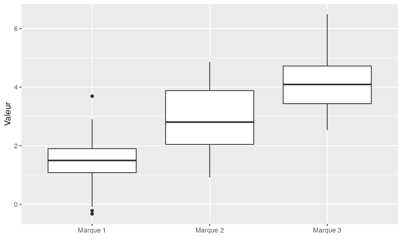

library(ggplot2)
ggplot(data=Marque.Valeur,aes(x=Marque,y=Valeur)) + geom_boxplot() + xlab("")

Chemin <- "~/Documents/Recherche/DeBoeck/Graphes/Donnees/"
colmodel="cmyk"
ggplot2::ggsave(filename = paste(Chemin,"MarqueValeur_boxplot.pdf",sep=""),
       width = 10, height = 7, onefile = TRUE, family = "Helvetica", title = "Boxplot", paper = "special", colormodel = colmodel)

options(contrasts = c("contr.sum","contr.sum"))
lm.Marque.Valeur <- lm(Valeur~Marque,data=Marque.Valeur)
anova(lm.Marque.Valeur)
#> Analysis of Variance Table
#> 
#> Response: Valeur
#>           Df  Sum Sq Mean Sq F value    Pr(>F)    
#> Marque     2 110.676  55.338  60.502 < 2.2e-16 ***
#> Residuals 87  79.575   0.915                      
#> ---
#> Signif. codes:  0 '***' 0.001 '**' 0.01 '*' 0.05 '.' 0.1 ' ' 1

-sum(coef(lm.Marque.Valeur)[2:3])
#> [1] 1.315667

res.model.MV <- residuals(lm.Marque.Valeur)
shapiro.test(res.model.MV)
#> 
#>  Shapiro-Wilk normality test
#> 
#> data:  res.model.MV
#> W = 0.98958, p-value = 0.6999

qqnorm(res.model.MV)
qqline(res.model.MV)

bartlett.test(res.model.MV,Marque.Valeur$Marque)
#> 
#>  Bartlett test of homogeneity of variances
#> 
#> data:  res.model.MV and Marque.Valeur$Marque
#> Bartlett's K-squared = 1.0505, df = 2, p-value = 0.5914

if(!("ggiraphExtra" %in% installed.packages())){install.packages("ggiraphExtra")}
library(ggiraphExtra)
Marque.Valeur$Marque<-as.factor(rep(paste("M",1:3),rep(rep(30,3))))
oav.Marque.Valeur <- aov(Valeur~Marque,data=Marque.Valeur)
resHSD <- TukeyHSD(oav.Marque.Valeur)
resHSD
#>   Tukey multiple comparisons of means
#>     95% family-wise confidence level
#> 
#> Fit: aov(formula = Valeur ~ Marque, data = Marque.Valeur)
#> 
#> $Marque
#>             diff       lwr      upr   p adj
#> M 2-M 1 1.478333 0.8895222 2.067144 1.0e-07
#> M 3-M 1 2.712667 2.1238555 3.301478 0.0e+00
#> M 3-M 2 1.234333 0.6455222 1.823144 8.8e-06

ggHSD(resHSD) + ylab("Differences entre les niveaux moyens de Marque") + ggtitle("Intervalles de confiance globale 95%")
#> Warning: `aes_string()` was deprecated in ggplot2 3.0.0.
#> ℹ Please use tidy evaluation idioms with `aes()`.
#> ℹ See also `vignette("ggplot2-in-packages")` for more information.
#> ℹ The deprecated feature was likely used in the ggiraphExtra package.
#>   Please report the issue to the authors.
#> This warning is displayed once every 8 hours.
#> Call `lifecycle::last_lifecycle_warnings()` to see where this warning was
#> generated.
#> Warning: Using `size` aesthetic for lines was deprecated in ggplot2 3.4.0.
#> ℹ Please use `linewidth` instead.
#> ℹ The deprecated feature was likely used in the ggiraphExtra package.
#>   Please report the issue to the authors.
#> This warning is displayed once every 8 hours.
#> Call `lifecycle::last_lifecycle_warnings()` to see where this warning was
#> generated.
#> Warning: The `<scale>` argument of `guides()` cannot be `FALSE`. Use "none" instead as
#> of ggplot2 3.3.4.
#> ℹ The deprecated feature was likely used in the ggiraphExtra package.
#>   Please report the issue to the authors.
#> This warning is displayed once every 8 hours.
#> Call `lifecycle::last_lifecycle_warnings()` to see where this warning was
#> generated.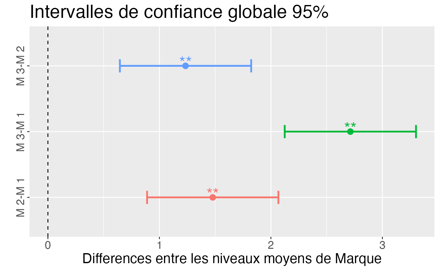

Chemin <- "~/Documents/Recherche/DeBoeck/Graphes/Donnees/"
colmodel="cmyk"
ggplot2::ggsave(filename = paste(Chemin,"MarqueValeur_Tukey.pdf",sep=""),
       width = 10, height = 7, onefile = TRUE, family = "Helvetica", title = "Boxplot", paper = "special", colormodel = colmodel)

C1=1+1/(3*(nlevels(Marque.Valeur$Marque)-1))*(sum(1/(table(Marque.Valeur$Marque)-1))-1/(nrow(Marque.Valeur)-nlevels(Marque.Valeur$Marque)))
C1
#> [1] 1.015326

1/C1*((nrow(Marque.Valeur)-nlevels(Marque.Valeur$Marque))*log(summary(oav.Marque.Valeur)[[1]]$`Mean Sq`[2])-sum((table(Marque.Valeur$Marque)-1)*log(with(Marque.Valeur,tapply(Valeur,Marque,var)))))
#> [1] 1.050525

bartlett.test(res.model.MV,Marque.Valeur$Marque)
#> 
#>  Bartlett test of homogeneity of variances
#> 
#> data:  res.model.MV and Marque.Valeur$Marque
#> Bartlett's K-squared = 1.0505, df = 2, p-value = 0.5914

QQplots

oldpar <- par()

Chemin <- "~/Documents/Recherche/DeBoeck/Graphes/"
colmodel="cmyk"
library(VGAM)

par(mar = c(0.2, 0.2, 0.2, 0.2) + 0.1, mgp = c(2, 1, 0))
ech_norm <- rnorm(100)
qqnorm(ech_norm, ylab="",main="", xaxt="n", yaxt="n")
legend("bottomright",legend="(a)",cex=2,bty="n")

pdf(file = paste(Chemin,"qqplota.pdf",sep=""),
    width = 8, height = 7, onefile = TRUE, family = "Helvetica",
    title = "QQplot", paper = "special")
par(mar = c(0.2, 0.2, 0.2, 0.2) + 0.1, mgp = c(2, 1, 0))
qqnorm(ech_norm, ylab="",main="", xaxt="n", yaxt="n")
legend("bottomright",legend="",cex=2,bty="n")
dev.off()
#> agg_png 
#>       2

par(mar = c(0.2, 0.2, 0.2, 0.2) + 0.1, mgp = c(2, 1, 0))
ech_laplace <- rlaplace(100,1/sqrt(2))
qqnorm(ech_laplace, ylab="",main="", xaxt="n", yaxt="n")
legend("bottomright",legend="(b)",cex=2,bty="n")

pdf(file = paste(Chemin,"qqplotb.pdf",sep=""),
    width = 8, height = 7, onefile = TRUE, family = "Helvetica",
    title = "QQplot ", paper = "special")
par(mar = c(0.2, 0.2, 0.2, 0.2) + 0.1, mgp = c(2, 1, 0))
qqnorm(ech_laplace, ylab="",main="", xaxt="n", yaxt="n")
legend("bottomright",legend="",cex=2,bty="n")
dev.off()
#> agg_png 
#>       2

par(mar = c(0.2, 0.2, 0.2, 0.2) + 0.1, mgp = c(2, 1, 0))
ech_unif <- runif(100,-2,2)
qqnorm(ech_unif, ylab="(c)",main="", xaxt="n", yaxt="n")
legend("bottomright",legend="(c)",cex=2,bty="n")

pdf(file = paste(Chemin,"qqplotc.pdf",sep=""),
    width = 8, height = 7, onefile = TRUE, family = "Helvetica",
    title = "QQplot ", paper = "special")
par(mar = c(0.2, 0.2, 0.2, 0.2) + 0.1, mgp = c(2, 1, 0))
qqnorm(ech_unif, ylab="",main="", xaxt="n", yaxt="n")
legend("bottomright",legend="",cex=2,bty="n")
dev.off()
#> agg_png 
#>       2

par(mar = c(0.2, 0.2, 0.2, 0.2) + 0.1, mgp = c(2, 1, 0))
ech_exp <- rexp(100,1)
qqnorm(ech_exp, ylab="",main="", xaxt="n", yaxt="n")
legend("bottomright",legend="(d)",cex=2,bty="n")

pdf(file = paste(Chemin,"qqplotd.pdf",sep=""),
    width = 8, height = 7, onefile = TRUE, family = "Helvetica",
    title = "QQplot ", paper = "special")
par(mar = c(0.2, 0.2, 0.2, 0.2) + 0.1, mgp = c(2, 1, 0))
qqnorm(ech_exp, ylab="",main="", xaxt="n", yaxt="n")
legend("bottomright",legend="",cex=2,bty="n")
dev.off()
#> agg_png 
#>       2

par(mar = c(0.2, 0.2, 0.2, 0.2) + 0.1, mgp = c(2, 1, 0))
ech_mel <- c(rnorm(50,0,1),rnorm(50,5,1))
qqnorm(ech_mel, ylab="", main="", xaxt="n", yaxt="n")
legend("bottomright",legend="(e)",cex=2,bty="n")

pdf(file = paste(Chemin,"qqplote.pdf",sep=""),
    width = 8, height = 7, onefile = TRUE, family = "Helvetica",
    title = "QQplot ", paper = "special")
par(mar = c(0.2, 0.2, 0.2, 0.2) + 0.1, mgp = c(2, 1, 0))
qqnorm(ech_mel, ylab="", main="", xaxt="n", yaxt="n")
legend("bottomright",legend="",cex=2,bty="n")
dev.off()
#> agg_png 
#>       2

par(mar = c(0.2, 0.2, 0.2, 0.2) + 0.1, mgp = c(2, 1, 0))
ech_ext <- c(rnorm(99,0),5)
qqnorm(ech_ext, ylab="",main="", xaxt="n", yaxt="n")
legend("bottomright",legend="(f)",cex=2,bty="n")

pdf(file = paste(Chemin,"qqplotf.pdf",sep=""),
    width = 8, height = 7, onefile = TRUE, family = "Helvetica",
    title = "QQplot ", paper = "special")
par(mar = c(0.2, 0.2, 0.2, 0.2) + 0.1, mgp = c(2, 1, 0))
qqnorm(ech_ext, ylab="",main="", xaxt="n", yaxt="n")
legend("bottomright",legend="",cex=2,bty="n")
dev.off()
#> agg_png 
#>       2

pdf(file = paste(Chemin,"qqplotall.pdf",sep=""),
    width = 8, height = 7, onefile = TRUE, family = "Helvetica",
    title = "QQplot ", paper = "special")
layout(matrix(1:6,nrow=2,byrow=T))
par(mar = c(0.2, 0.2, 0.2, 0.2) + 0.1, mgp = c(2, 1, 0))
qqnorm(ech_norm, ylab="",main="", xaxt="n", yaxt="n")
legend("bottomright",legend="(a)",cex=2,bty="n")
par(mar = c(0.2, 0.2, 0.2, 0.2) + 0.1, mgp = c(2, 1, 0))
qqnorm(ech_laplace, ylab="",main="", xaxt="n", yaxt="n")
legend("bottomright",legend="(b)",cex=2,bty="n")
par(mar = c(0.2, 0.2, 0.2, 0.2) + 0.1, mgp = c(2, 1, 0))
qqnorm(ech_unif, ylab="",main="", xaxt="n", yaxt="n")
legend("bottomright",legend="(c)",cex=2,bty="n")
par(mar = c(0.2, 0.2, 0.2, 0.2) + 0.1, mgp = c(2, 1, 0))
qqnorm(ech_exp, ylab="",main="", xaxt="n", yaxt="n")
legend("bottomright",legend="(d)",cex=2,bty="n")
par(mar = c(0.2, 0.2, 0.2, 0.2) + 0.1, mgp = c(2, 1, 0))
qqnorm(ech_mel, ylab="", main="", xaxt="n", yaxt="n")
legend("bottomright",legend="(e)",cex=2,bty="n")
par(mar = c(0.2, 0.2, 0.2, 0.2) + 0.1, mgp = c(2, 1, 0))
qqnorm(ech_ext, ylab="",main="", xaxt="n", yaxt="n")
legend("bottomright",legend="(f)",cex=2,bty="n")
dev.off()
#> agg_png 
#>       2

Tout le code avec R.

F. Bertrand et M. Maumy

2025-09-22

Intervalles de confiance

Pour la moyenne

Pour la variance

Test $t$ pour un échantillon

Test $t$ pour deux échantillons indépendants.

Test $t$ pour deux échantillons appariés

Analyse de la variance à un facteur

QQplots

Chapitre 09. Inférence statistique.

Tout le code avec R.

F. Bertrand et M. Maumy

2025-09-22

Intervalles de confiance

Pour la moyenne

Pour la variance

Test tt pour un échantillon

Test tt pour deux échantillons indépendants.

Test tt pour deux échantillons appariés

Analyse de la variance à un facteur

QQplots

Test $t$ pour un échantillon

Test $t$ pour deux échantillons indépendants.

Test $t$ pour deux échantillons appariés