Chapitre 03. Statistiques descriptives et visualisation des données bivariables ou multivariables.
Tout le code avec R.
F. Bertrand et M. Maumy
2025-09-22
Source:vignettes/CodeChap03.Rmd
CodeChap03.Rmd

|
|
Sources des données
Statistique Canada
Données libres d’utilisation, commerciale ou non, sur Statistique Canada. https://www.statcan.gc.ca/fra/reference/droit-auteur
répartition en classes d’âge de la population du Canada en 2020. Statistique Canada. Tableau 17-10-0005-01 Estimations de la population au 1er juillet, par âge et sexe DOI : https://doi.org/10.25318/1710000501-fra
population des dix provinces et trois territoires du Canada au quatrième trimestre 2020. Source : Statistique Canada. Tableau 17-10-0009-01. Estimations de la population, trimestrielles. DOI : https://doi.org/10.25318/1710000901-fra
Statistique de l’OCDE.
- Taux d’emploi en % de la classe d’age
Taux d’emploi par groupe d’âge (indicateur). OCDE (2021). doi: 10.1787/b01db125-fr (Consulté le 11 février 2021)
Le taux d’emploi d’une classe d’âge se mesure en fonction du nombre des actifs occupés d’un âge donné rapporté à l’effectif total de cette classe d’âge. Les actifs occupés sont les personnes de 15 ans et plus qui, durant la semaine de référence, déclarent avoir effectué un travail rémunéré pendant une heure au moins ou avoir occupé un emploi dont elles étaient absentes. Les taux d’emploi sont présentés pour quatre classes d’âge : les personnes âgées de 15 à 64 ans (personnes en âge de travailler); les personnes âgées de 15 à 24 ans sont celles qui font leur entrée sur le marché du travail à l’issue de leur scolarité, les personnes âgées de 25 à 54 ans sont celles qui sont au plus fort de leur activité professionnelle, et les personnes âgées de 55 à 64 ans sont celles qui ont dépassé le pic de leur carrière professionnelle et approchent de l’âge de la retraite. Cet indicateur est désaisonnalisé et est mesuré en pourcentage de l’effectif total de la classe d’âge.
- Par secteur dans les pays de l’OCDE en 2020-Q3.
Emploi par activité (indicateur). OCDE (2021). doi: 10.1787/6b2fff89-fr (Consulté le 11 février 2021)
- Emploi par niveau d’études en % des 25-64 ans
Emploi par niveau d’études (indicateur). OCDE (2021) doi: 10.1787/6e3d44f3-fr (Consulté le 11 février 2021)
Cet indicateur fournit les taux d’emploi selon le niveau d’études : premier cycle du second degré, deuxième cycle du second degré, supérieur. Le taux d’emploi est le pourcentage d’actifs occupés dans la population en âge de travailler. Les actifs occupés sont les personnes qui travaillent au moins une heure par semaine en tant que salarié ou à titre lucratif, ou qui ont un emploi mais sont temporairement absentes de leur travail pour maladie, congé ou conflit social. Cet indicateur donne le pourcentage des actifs occupés âgés de 25 à 64 ans dans la population des individus âgés de 25 à 64 ans.
- Part du revenu national total équivalent en Euro en 2019. Répartitition du revenu par quantiles - enquêtes EU-SILC et PCM (ILC_DI01).
INSEE
- Ménages par taille du ménage,
MEN4 - Ménages par taille du ménage, sexe et âge de la personne de référence en 2017. France métropolitaine. Insee.
Données Covid officielles
Répartition par région française du nombre de personnes hospitalisées et atteintes du Covid 19 le 21 février 2021.
Répartition par région française du nombre de personne en réanimation et atteintes du Covid 19 le 21 février 2021.
if(!("sageR" %in% installed.packages())){install.packages("sageR")}
library(sageR)
Distribution conjointe
data(Europe)
Europe
#>        Etats.membres Partiel_Ens Partiel_H Partiel_F Salariés NonSalariés
#> 1          Allemagne        27.2       9.9      46.7     40.2        47.6
#> 2           Autriche        27.2       9.5      47.1     41.1        51.2
#> 3           Belgique        24.9      10.5      41.0     39.1        52.5
#> 4           Bulgarie         1.9       1.7       2.1     40.7        43.0
#> 5             Chypre        10.2       6.3      14.6     41.2        44.9
#> 6            Croatie         4.8       3.1       6.7     40.4        44.6
#> 7           Danemark        24.2      15.3      33.9     37.6        46.3
#> 8            Espagne        14.5       6.8      23.7     39.6        47.0
#> 9            Estonie        11.3       7.1      15.9     40.2        43.2
#> 10          Finlande        15.5      10.1      21.3     39.4        46.4
#> 11            France        17.5       7.5      28.0     39.1        50.1
#> 12             Grèce         9.1       5.9      13.5     40.7        50.4
#> 13           Hongrie         4.4       2.5       6.8     40.4        41.5
#> 14           Irlande        19.7      10.1      30.6     39.4        49.4
#> 15           Islande        21.5      10.3      34.1     43.4        48.5
#> 16            Italie        18.7       8.2      32.9     39.0        46.0
#> 17          Lettonie         8.4       5.8      10.9     40.2        41.5
#> 18          Lituanie         6.4       4.7       8.0     39.9        40.6
#> 19        Luxembourg        17.0       5.6      30.4     40.2        46.9
#> 20 Macédoine du Nord         4.1       4.1       4.3     41.6        45.3
#> 21             Malte        12.2       5.9      21.4     41.3        47.4
#> 22        Monténégro         4.5       4.7       4.1     44.6        48.3
#> 23           Norvège        25.8      15.2      37.7     38.4        45.0
#> 24          Pays-Bas        50.2      27.9      75.2     38.9        47.9
#> 25           Pologne         6.1       3.5       9.3     40.8        45.7
#> 26          Portugal         8.1       5.4      10.9     40.8        47.6
#> 27          Roumanie         6.1       6.0       6.2     40.6        38.9
#> 28       Royaume-Uni        24.4      10.8      39.4     42.0        45.2
#> 29            Serbie         9.7       8.9      10.6     42.8        51.2
#> 30         Slovaquie         4.5       2.9       6.5     40.5        45.1
#> 31          Slovénie         8.4       4.8      12.7     40.7        45.7
#> 32             Suède        22.5      13.4      32.5     39.9        47.9
#> 33            Suisse        38.0      17.1      61.7     41.8        49.4
#> 34          Tchéquie         6.3       2.8      10.6     40.7        45.9
#> 35           Turquie         9.9       6.6      17.0     48.1        49.6
Salariés*Non-salariés
SalXNsal=table(cut(Europe$Salariés,c(35,40,45)),cut(Europe$NonSalariés,c(35,40,45,50,55)))
prop.table(SalXNsal)
#>
#>              (35,40]    (40,45]    (45,50]    (50,55]
#>   (35,40] 0.00000000 0.05882353 0.20588235 0.05882353
#>   (40,45] 0.02941176 0.17647059 0.38235294 0.08823529

tabSXNs1=margin.table(SalXNsal,1)
round(tabSXNs1,digits=2)
#>
#> (35,40] (40,45]
#>      11      23
tabSXNs2=margin.table(SalXNsal,2)
round(tabSXNs2,digits=2)
#>
#> (35,40] (40,45] (45,50] (50,55]
#>       1       8      20       5
tabSXNs3=margin.table(SalXNsal,1)/sum(SalXNsal)
round(tabSXNs3,digits=2)
#>
#> (35,40] (40,45]
#>    0.32    0.68
tabSXNs4=margin.table(SalXNsal,2)/sum(SalXNsal)
round(tabSXNs4,digits=2)
#>
#> (35,40] (40,45] (45,50] (50,55]
#>    0.03    0.24    0.59    0.15
tabSXNs5=prop.table(SalXNsal,1)
round(tabSXNs5,digits=2)
#>
#>           (35,40] (40,45] (45,50] (50,55]
#>   (35,40]    0.00    0.18    0.64    0.18
#>   (40,45]    0.04    0.26    0.57    0.13

tabSXNs7=prop.table(SalXNsal,2)
round(tabSXNs7,digits=2)
#>
#>           (35,40] (40,45] (45,50] (50,55]
#>   (35,40]    0.00    0.25    0.35    0.40
#>   (40,45]    1.00    0.75    0.65    0.60
Temps partiel Hommes*Femmes
HomXFem=table(cut(Europe$Partiel_H,c(0,10,20,30)),cut(Europe$Partiel_F,c(0,10,20,30,40,50,60,70,80)))
HomXFem
#>
#>           (0,10] (10,20] (20,30] (30,40] (40,50] (50,60] (60,70] (70,80]
#>   (0,10]       9       9       3       2       2       0       0       0
#>   (10,20]      0       0       1       6       1       0       1       0
#>   (20,30]      0       0       0       0       0       0       0       1
prop.table(HomXFem)
#>
#>               (0,10]    (10,20]    (20,30]    (30,40]    (40,50]    (50,60]
#>   (0,10]  0.25714286 0.25714286 0.08571429 0.05714286 0.05714286 0.00000000
#>   (10,20] 0.00000000 0.00000000 0.02857143 0.17142857 0.02857143 0.00000000
#>   (20,30] 0.00000000 0.00000000 0.00000000 0.00000000 0.00000000 0.00000000
#>
#>              (60,70]    (70,80]
#>   (0,10]  0.00000000 0.00000000
#>   (10,20] 0.02857143 0.00000000
#>   (20,30] 0.00000000 0.02857143

tabHXFs1=margin.table(HomXFem,1)
round(tabHXFs1,digits=2)
#>
#>  (0,10] (10,20] (20,30]
#>      25       9       1
tabHXFs2=margin.table(HomXFem,2)
round(tabHXFs2,digits=2)
#>
#>  (0,10] (10,20] (20,30] (30,40] (40,50] (50,60] (60,70] (70,80]
#>       9       9       4       8       3       0       1       1
tabHXFs3=margin.table(HomXFem,1)/sum(HomXFem)
round(tabHXFs3,digits=2)
#>
#>  (0,10] (10,20] (20,30]
#>    0.71    0.26    0.03
tabHXFs4=margin.table(HomXFem,2)/sum(HomXFem)
round(tabHXFs4,digits=2)
#>
#>  (0,10] (10,20] (20,30] (30,40] (40,50] (50,60] (60,70] (70,80]
#>    0.26    0.26    0.11    0.23    0.09    0.00    0.03    0.03
tabHXFs5=prop.table(HomXFem,1)
round(tabHXFs5,digits=2)
#>
#>           (0,10] (10,20] (20,30] (30,40] (40,50] (50,60] (60,70] (70,80]
#>   (0,10]    0.36    0.36    0.12    0.08    0.08    0.00    0.00    0.00
#>   (10,20]   0.00    0.00    0.11    0.67    0.11    0.00    0.11    0.00
#>   (20,30]   0.00    0.00    0.00    0.00    0.00    0.00    0.00    1.00

tabHXFs7=prop.table(HomXFem,2)
round(tabHXFs7,digits=2)
#>
#>           (0,10] (10,20] (20,30] (30,40] (40,50] (50,60] (60,70] (70,80]
#>   (0,10]    1.00    1.00    0.75    0.25    0.67            0.00    0.00
#>   (10,20]   0.00    0.00    0.25    0.75    0.33            1.00    0.00
#>   (20,30]   0.00    0.00    0.00    0.00    0.00            0.00    1.00
Représentation série double
OCDE Secteur (Quali-Quali)
data(Secteur)

rownames(Secteur) <- Secteur$PAYS
Secteur <- as.table(as.matrix(round(Secteur[,-1]*1000)))

margin.table(Secteur)
#> [1] 594711234
margin.table(Secteur,1)
#>       AUT       BEL       CAN       CHE       CHL       COL       CZE       DNK
#>   5337903   5721200  21122321   5568900   8732089  22791085   7015674   3343269
#>       ESP       EST       FIN       FRA       GBR       GRC       HUN       IRL
#>  22701902    200240   1154495  31775373  37353540   4382010   5787638   2692289
#>       ISL       ISR       ITA       JPN       KOR       LTU       LUX       LVA
#>     40221   4366750  28409214  81977909  33262656   1647480    316889    253516
#>       NLD       NOR       NZL       POL       PRT       SVK       SVN       SWE
#>  10143659   3114348   3242630  21006175   5902090   3385345   1275598   5872256
#>       TUR       USA
#>  33604952 171209618
margin.table(Secteur,2)
#>         AGR      CONSTR INDUSCONSTR         MFG        SERV
#>    21143584    35197834   105139612    64298384   368931820
oldpar <- par()
margX <- margin.table(Secteur,1)
par(mar = c(3, 3, 1, 1) + 0.1, mgp = c(2, 1, 0))
mp <- barplot(margX, beside=FALSE, args.legend=list(x="topright"),col=c("black","cyan","black","cyan"),density=25) # default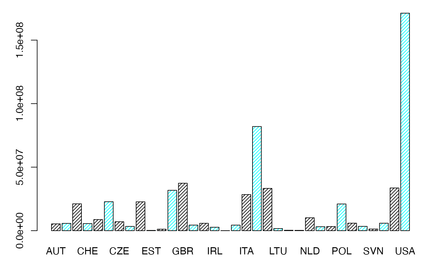
margY <- margin.table(Secteur,2)
par(mar = c(3, 3, 1, 1) + 0.1, mgp = c(2, 1, 0))
mp <- barplot(margY, beside=FALSE, args.legend=list(x="topright"),col=c("black","cyan","black","cyan"),density=25) # default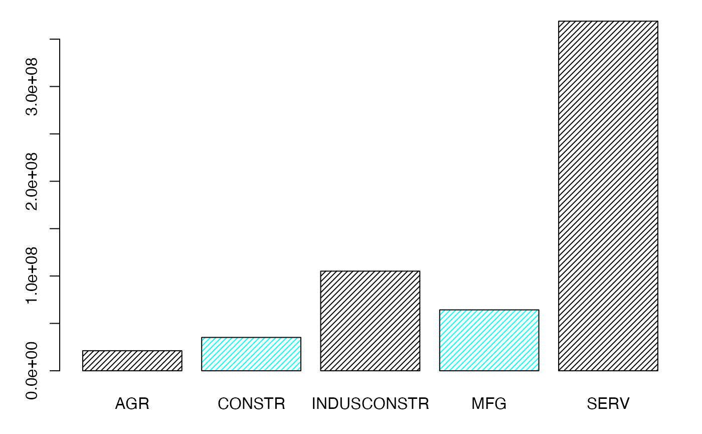
layout((1:2))
margX <- margin.table(Secteur,1)
par(mar = c(3, 3, 1, 1) + 0.1, mgp = c(2, 1, 0))
mp <- barplot(margX, beside=FALSE, args.legend=list(x="topright"),col=c("black","cyan","black","cyan"),density=25,las=2) # default
margY <- margin.table(Secteur,2)
par(mar = c(3, 3, 1, 1) + 0.1, mgp = c(2, 1, 0))
mp <- barplot(margY, beside=FALSE, args.legend=list(x="topright"),col=c("black","cyan","black","cyan"),density=25) # default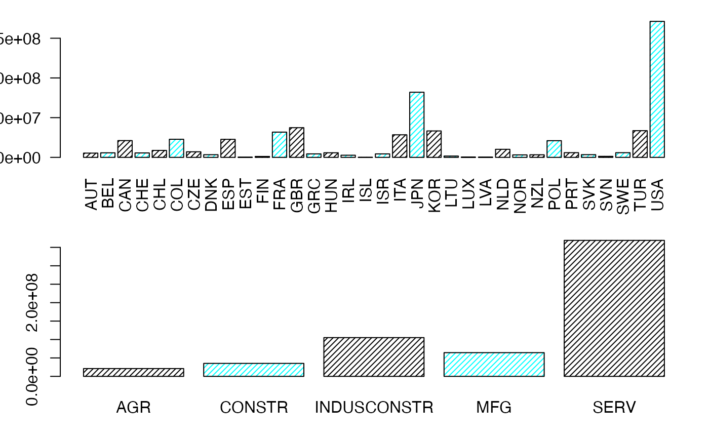
Chemin <- "~/Documents/Recherche/DeBoeck/Graphes/Fichiers/"
colmodel="cmyk"
pdf(file = "effmargX.pdf",
    width = 8, height = 7, onefile = TRUE, family = "Helvetica",
    title = "Probability or cumulative distribution graphs", paper = "special", colormodel = colmodel)
layout((1:2))
margX <- margin.table(Secteur,1)
par(mar = c(3, 3, 1, 1) + 0.1, mgp = c(2, 1, 0))
mp <- barplot(margX, beside=FALSE, args.legend=list(x="topright"),col=c("black","cyan","black","cyan"),density=25,las=2) # default
margY <- margin.table(Secteur,2)
par(mar = c(3, 3, 1, 1) + 0.1, mgp = c(2, 1, 0))
mp <- barplot(margY, beside=FALSE, args.legend=list(x="topright"),col=c("black","cyan","black","cyan"),density=25) # default
dev.off()
#> agg_png
#>       2
layout(1)
freqcondY <- prop.table(Secteur,2) #Y|X
par(mar = c(3, 3, 1, 1) + 0.1, mgp = c(2, 1, 0))
mp <- barplot(freqcondY, beside=TRUE, legend = rownames(Secteur), ylim = c(0, .5), args.legend=list(x="top", ncol=7)) # default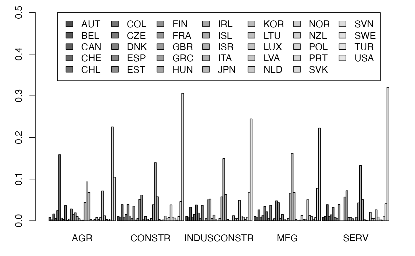
freqcondX <- prop.table(Secteur,1) #Y|X
par(mar = c(3, 3, 1, 1) + 0.1, mgp = c(2, 1, 0))
mp <- barplot(t(freqcondX), beside=TRUE, legend = colnames(Secteur), ylim = c(0, 1.05), args.legend=list(x="top", ncol=3),las=2) # default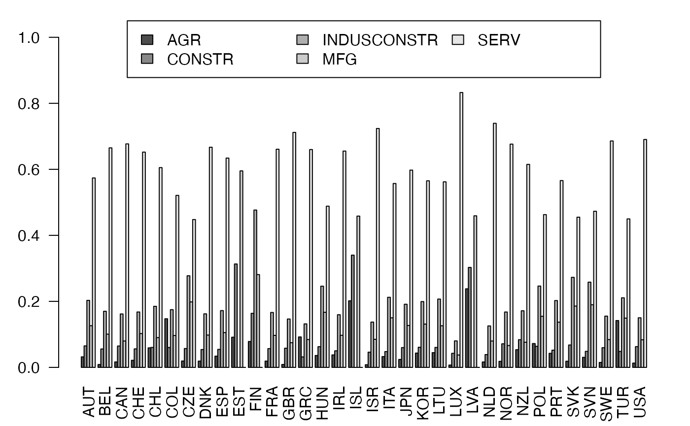
Chemin <- "~/Documents/Recherche/DeBoeck/Graphes/Fichiers/"
colmodel="cmyk"
pdf(file = "frecondBesideY.pdf",
    width = 8, height = 7, onefile = TRUE, family = "Helvetica",
    title = "Probability or cumulative distribution graphs", paper = "special", colormodel = colmodel)
layout(1)
freqcondY <- prop.table(Secteur,2) #Y|X
par(mar = c(3, 3, 1, 1) + 0.1, mgp = c(2, 1, 0))
mp <- barplot(freqcondY, beside=TRUE, legend = rownames(Secteur), ylim = c(0, .4), args.legend=list(x="top", ncol=7)) # default
dev.off()
#> agg_png
#>       2

pdf(file = "frecondBesideX.pdf",
    width = 8, height = 7, onefile = TRUE, family = "Helvetica",
    title = "Probability or cumulative distribution graphs", paper = "special", colormodel = colmodel)
layout(1)
freqcondX <- prop.table(Secteur,1) #Y|X
par(mar = c(3, 3, 1, 1) + 0.1, mgp = c(2, 1, 0))
mp <- barplot(t(freqcondX), beside=TRUE, legend = colnames(Secteur), ylim = c(0, 0.95), args.legend=list(x="top", ncol=3),las=2) # default
dev.off()
#> agg_png
#>       2
layout(1)
freqcondY <- prop.table(Secteur,2) #Y|X
par(mar = c(3, 3, 1, 1) + 0.1, mgp = c(2, 1, 0))
mp <- barplot(freqcondY, beside=FALSE, legend = rownames(Secteur), ylim = c(0, 1.6), args.legend=list(x="top", ncol=7),yaxt="n") # default
axis(2, at=0:5*.2)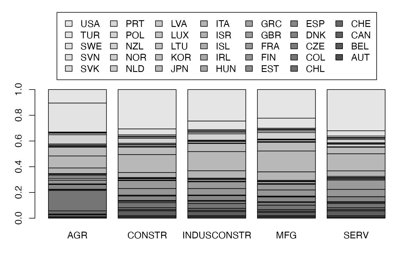
freqcondX <- prop.table(Secteur,1) #Y|X
par(mar = c(3, 3, 1, 1) + 0.1, mgp = c(2, 1, 0))
mp <- barplot(t(freqcondX), beside=FALSE, legend = colnames(Secteur), ylim = c(0, 1.3), args.legend=list(x="top", ncol=3),yaxt="n",las=2) # default
axis(2, at=0:5*.2)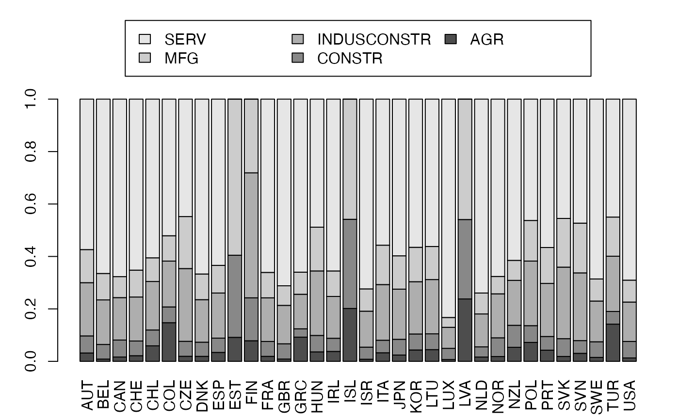
Chemin <- "~/Documents/Recherche/DeBoeck/Graphes/Fichiers/"
colmodel="cmyk"
pdf(file = "frecondStacked_Y.pdf",
    width = 8, height = 7, onefile = TRUE, family = "Helvetica",
    title = "Probability or cumulative distribution graphs", paper = "special", colormodel = colmodel)
layout(1)
freqcondY <- prop.table(Secteur,2) #Y|X
par(mar = c(3, 3, 1, 1) + 0.1, mgp = c(2, 1, 0))
mp <- barplot(freqcondY, beside=FALSE, legend = rownames(Secteur), ylim = c(0, 1.4), args.legend=list(x="top", ncol=7),yaxt="n") # default
axis(2, at=0:5*.2)

pdf(file = "frecondStacked_X.pdf",
    width = 8, height = 7, onefile = TRUE, family = "Helvetica",
    title = "Probability or cumulative distribution graphs", paper = "special", colormodel = colmodel)
freqcondX <- prop.table(Secteur,1) #Y|X
par(mar = c(3, 3, 1, 1) + 0.1, mgp = c(2, 1, 0))
mp <- barplot(t(freqcondX), beside=FALSE, legend = colnames(Secteur), ylim = c(0, 1.2), args.legend=list(x="top", ncol=3),yaxt="n",las=2) # default
axis(2, at=0:5*.2)
dev.off()
#> agg_png
#>       2
Salariés*Non-salariés (Quanti-Quanti)
data(Europe)
table(cut(Europe$Salariés,c(35,40,45,50)))
#>
#> (35,40] (40,45] (45,50]
#>      11      23       1
table(cut(Europe$NonSalariés,c(35,40,45,50,55)))
#>
#> (35,40] (40,45] (45,50] (50,55]
#>       1       8      21       5
Distribution conditionnelle
ff=table(cut(Europe$Salariés,c(35,40,45,50)),
cut(Europe$NonSalariés,c(35,40,45,50,55)))/sum(table(cut(Europe$Salariés,c(35,40,45,50)),cut(Europe$NonSalariés,c(35,40,45,50,55))))
if(!("lattice" %in% installed.packages())){install.packages("lattice")}
library(lattice)
freqcondX <- prop.table(ff,1) #Y|X
freqcondY <- prop.table(ff,2) #Y|X
ensemble.df <- make.groups(freqcondX)
colnames(ensemble.df) <- c("Taux","ClasseX")
ensemble.df$ClasseX <- rep(colnames(ff),rep(3,length(colnames(ff))))
ensemble.df$ClasseY <- rep(rownames(ff),length(colnames(ff)))
ensemble.df
#>                   Taux ClasseX ClasseY
#> freqcondX1  0.00000000 (35,40] (35,40]
#> freqcondX2  0.04347826 (35,40] (40,45]
#> freqcondX3  0.00000000 (35,40] (45,50]
#> freqcondX4  0.18181818 (40,45] (35,40]
#> freqcondX5  0.26086957 (40,45] (40,45]
#> freqcondX6  0.00000000 (40,45] (45,50]
#> freqcondX7  0.63636364 (45,50] (35,40]
#> freqcondX8  0.56521739 (45,50] (40,45]
#> freqcondX9  1.00000000 (45,50] (45,50]
#> freqcondX10 0.18181818 (50,55] (35,40]
#> freqcondX11 0.13043478 (50,55] (40,45]
#> freqcondX12 0.00000000 (50,55] (45,50]
freqmargtempspartiel.pdf
Salariés<-Europe$Partiel_H
NonSalariés<-Europe$Partiel_F
Ensemble.df <- make.groups(Salariés,NonSalariés)
colnames(Ensemble.df) <- c("Taux","Genre")
Séparément
par(mar = c(3, 3, 1, 1) + 0.1, mgp = c(2, 1, 0))
histogram(Salariés,xlab="Temps partiels (% emploi total)",breaks=c(0,10,20,30,40,50,60,70,80))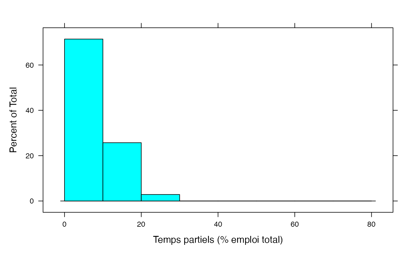
par(mar = c(3, 3, 1, 1) + 0.1, mgp = c(2, 1, 0))
histogram(NonSalariés,xlab="Temps partiels (% emploi total)",breaks=c(0,10,20,30,40,50,60,70,80))
Les deux ensemble
par(mar = c(3, 3, 1, 1) + 0.1, mgp = c(2, 1, 0))
histogram(~Taux|Genre,xlab="Temps partiels (% emploi total)",data=Ensemble.df,breaks=c(0,10,20,30,40,50,60,70,80),layout=c(1,2))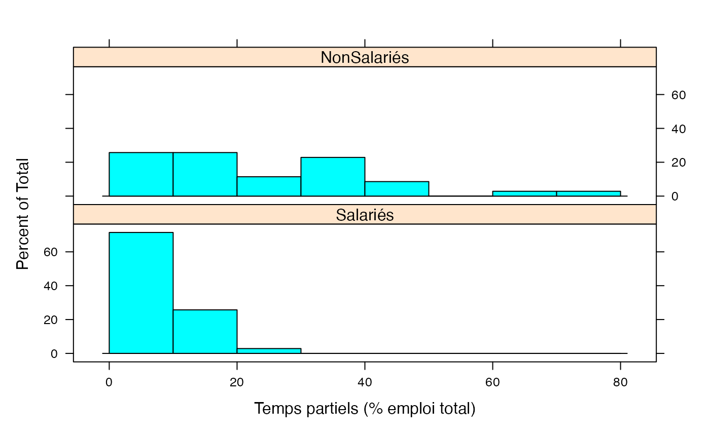
Chemin <- "~/Documents/Recherche/DeBoeck/Graphes/Fichiers/"
colmodel="cmyk"
pdf(file = "SNSfreqmargtempspartiel.pdf",
    width = 8, height = 7, onefile = TRUE, family = "Helvetica",
    title = "Probability or cumulative distribution graphs", paper = "special", colormodel = colmodel)
par(mar = c(3, 3, 1, 1) + 0.1, mgp = c(2, 1, 0))
histogram(~Taux|Genre,xlab="Temps partiels (% emploi total)",data=Ensemble.df,breaks=c(0,10,20,30,40,50,60,70,80),layout=c(1,2))
dev.off()
#> agg_png
#>       2
tfreqmargtempspartiel.pdf
par(mar = c(3, 3, 1, 1) + 0.1, mgp = c(2, 1, 0))
histogram(~Taux|Genre,xlab="Temps partiels (% emploi total)",data=Ensemble.df,breaks=c(0,10,20,30,40,50,60,70,80))
Chemin <- "~/Documents/Recherche/DeBoeck/Graphes/Fichiers/"
colmodel="cmyk"
pdf(file = "SNStfreqmargtempspartiel.pdf",
    width = 8, height = 7, onefile = TRUE, family = "Helvetica",
    title = "Probability or cumulative distribution graphs", paper = "special", colormodel = colmodel)
par(mar = c(3, 3, 1, 1) + 0.1, mgp = c(2, 1, 0))
histogram(~Taux|Genre,xlab="Temps partiels (% emploi total)",data=Ensemble.df,breaks=c(0,10,20,30,40,50,60,70,80))
dev.off()
#> agg_png
#>       2
freqcondX.pdf
#mp <- barplot(t(freqcondX),legend = rownames(freqcondX), ylim = c(0, 1)) # default
par(mar = c(3, 3, 1, 1) + 0.1, mgp = c(2, 1, 0))
mp <- barplot(t(freqcondX), beside=TRUE, legend = colnames(freqcondX), ylim = c(0, 1), args.legend=list(x="topleft",ncol=2,title="Non-salariés"),ylab="Pourcentage du total",xlab="Salariés") # default
#text(mp, t(freqcondX)+.05, format(freqcondX,digits=2), xpd = TRUE, col = "blue")
mtext(0:4*20,at=c(1+2*0:4),side=1)
mtext(0:4*20,at=c(10+2*0:4),side=1)
mtext(0:4*20,at=c(19+2*0:4),side=1)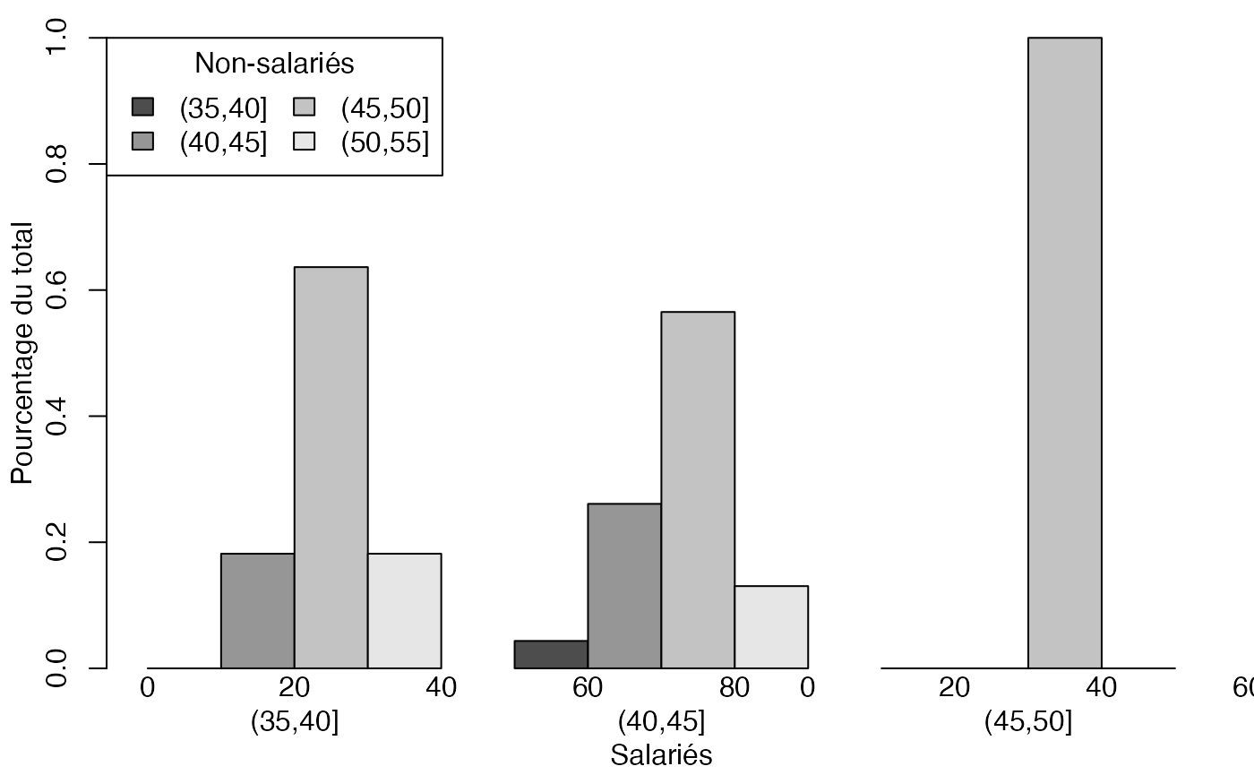
Chemin <- "~/Documents/Recherche/DeBoeck/Graphes/Fichiers/"
colmodel="cmyk"
pdf(file = "SNSfreqcondX.pdf",
    width = 8, height = 7, onefile = TRUE, family = "Helvetica",
    title = "Probability or cumulative distribution graphs", paper = "special", colormodel = colmodel)
par(mar = c(3, 3, 1, 1) + 0.1, mgp = c(2, 1, 0))
mp <- barplot(t(freqcondX), beside=TRUE, legend = colnames(freqcondX), ylim = c(0, 1), args.legend=list(x="topleft",ncol=2,title="Non-salariés"),ylab="Pourcentage du total",xlab="Salariés") # default
#text(mp, t(freqcondX)+.05, format(freqcondX,digits=2), xpd = TRUE, col = "blue")
mtext(0:4*20,at=c(1+2*0:4),side=1)
mtext(0:4*20,at=c(10+2*0:4),side=1)
mtext(0:4*20,at=c(19+2*0:4),side=1)
dev.off()
#> agg_png
#>       2
freqcondY.pdf
#mp <- barplot(t(freqcondX),legend = rownames(freqcondX), ylim = c(0, 1)) # default
par(mar = c(3, 3, 1, 1) + 0.1, mgp = c(2, 1, 0))
mp <- barplot(freqcondY, beside=TRUE, legend = rownames(freqcondY), ylim = c(0, 1), args.legend=list(x="top",ncol=3,title="Salariés"),ylab="Pourcentage du total",xlab="Non-salariés") # default
#text(mp, t(freqcondX)+.05, format(freqcondX,digits=2), xpd = TRUE, col = "blue")
mtext(0:1*20,at=c(1+2*0:1),side=1)
mtext(0:1*20,at=c(5+2*0:1),side=1)
mtext(0:1*20,at=c(9+2*0:1),side=1)
mtext(0:1*20,at=c(13+2*0:1),side=1)
mtext(0:1*20,at=c(17+2*0:1),side=1)
mtext(0:1*20,at=c(21+2*0:1),side=1)
mtext(0:1*20,at=c(25+2*0:1),side=1)
mtext(0:1*20,at=c(29+2*0:1),side=1)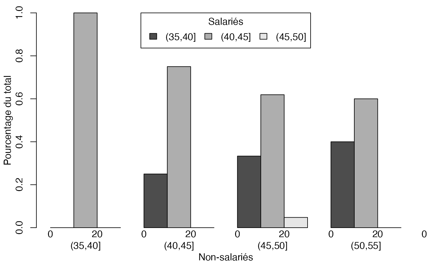
Chemin <- "~/Documents/Recherche/DeBoeck/Graphes/Fichiers/"
colmodel="cmyk"
pdf(file = "SNSfreqcondY.pdf",
    width = 8, height = 7, onefile = TRUE, family = "Helvetica",
    title = "Probability or cumulative distribution graphs", paper = "special", colormodel = colmodel)
#mp <- barplot(t(freqcondX),legend = rownames(freqcondX), ylim = c(0, 1)) # default
par(mar = c(3, 3, 1, 1) + 0.1, mgp = c(2, 1, 0))
mp <- barplot(freqcondY, beside=TRUE, legend = rownames(freqcondY), ylim = c(0, 1), args.legend=list(x="top",ncol=3,title="Salariés"),ylab="Pourcentage du total",xlab="Non-salariés")  # default
#text(mp, t(freqcondX)+.05, format(freqcondX,digits=2), xpd = TRUE, col = "blue")
mtext(0:1*20,at=c(1+2*0:1),side=1)
mtext(0:1*20,at=c(5+2*0:1),side=1)
mtext(0:1*20,at=c(9+2*0:1),side=1)
mtext(0:1*20,at=c(13+2*0:1),side=1)
mtext(0:1*20,at=c(17+2*0:1),side=1)
mtext(0:1*20,at=c(21+2*0:1),side=1)
mtext(0:1*20,at=c(25+2*0:1),side=1)
mtext(0:1*20,at=c(29+2*0:1),side=1)
dev.off()
#> agg_png
#>       2
disptempspartiel.pdf
par(mar = c(3, 3, 1, 1) + 0.1, mgp = c(2, 1, 0))
plot(Europe$Salariés,Europe$NonSalariés,xlab="Salariés",ylab="Non-salariés",pch=19)
colmodel="cmyk"
Chemin <- "~/Documents/Recherche/DeBoeck/Graphes/Fichiers/"
colmodel="cmyk"
pdf(file = "SNSdisptempspartiel.pdf",
    width = 8, height = 7, onefile = TRUE, family = "Helvetica",
    title = "Probability or cumulative distribution graphs", paper = "special", colormodel = colmodel)
par(mar = c(3, 3, 1, 1) + 0.1, mgp = c(2, 1, 0))
plot(Europe$Salariés,Europe$NonSalariés,xlab="Salariés",ylab="Non-salariés",pch=19)
dev.off()
#> agg_png
#>       2
stereotempspartiel.pdf
ff=table(cut(Europe$Partiel_H,c(0,10,20,30)),cut(Europe$Partiel_F,c(0,10,20,30,40,50,60,70,80)))/sum(table(cut(Europe$Partiel_H,c(0,10,20,30)),cut(Europe$Partiel_F,c(0,10,20,30,40,50,60,70,80))))
plotcdf3(c(0,10,20,30),c(0,10,20,30,40,50,60,70,80),f=ff,xaxe="Salariés",yaxe="Non-salariés",theme="0")
plotcdf3(c(0,10,20,30),c(0,10,20,30,40,50,60,70,80),f=ff,xaxe="Salariés",yaxe="Non-salariés",theme="1")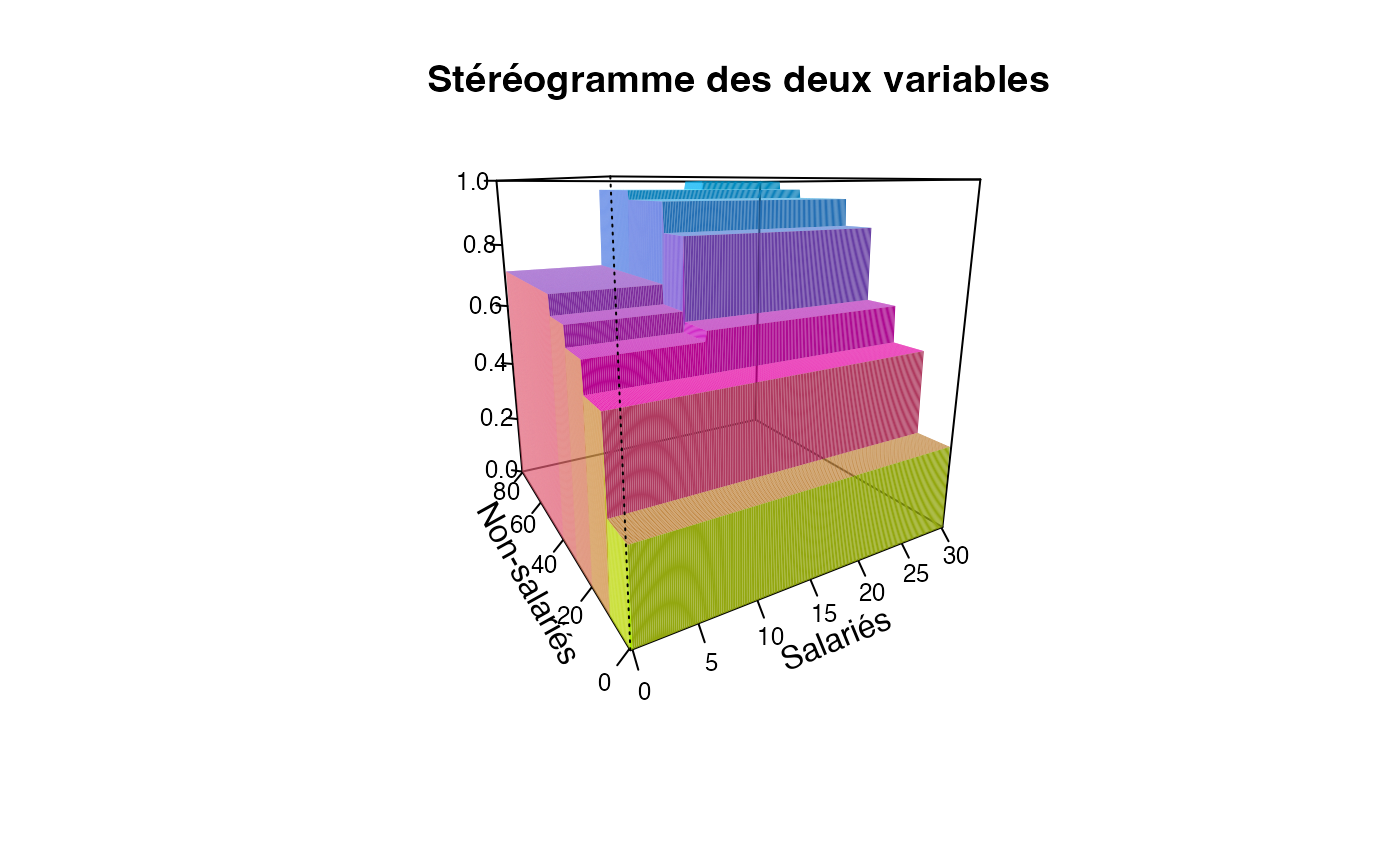
plotcdf3(c(0,10,20,30),c(0,10,20,30,40,50,60,70,80),f=ff,xaxe="Salariés",yaxe="Non-salariés",theme="2")
plotcdf3(c(0,10,20,30),c(0,10,20,30,40,50,60,70,80),f=ff,xaxe="Salariés",yaxe="Non-salariés",theme="cyan")
plotcdf3(c(0,10,20,30),c(0,10,20,30,40,50,60,70,80),f=ff,xaxe="Salariés",yaxe="Non-salariés",theme="cyan",border=TRUE)
plotcdf3(c(0,10,20,30),c(0,10,20,30,40,50,60,70,80),f=ff,xaxe="Salariés",yaxe="Non-salariés",theme="bw")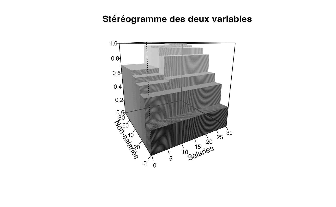
Chemin <- "~/Documents/Recherche/DeBoeck/Graphes/Fichiers/"
colmodel="cmyk"
pdf(file = "SNSstereotempspartiel.pdf",
    width = 8, height = 7, onefile = TRUE, family = "Helvetica",
    title = "Probability or cumulative distribution graphs", paper = "special", colormodel = colmodel)
par(mar = c(3, 3, 1, 1) + 0.1, mgp = c(2, 1, 0))
plotcdf3(c(0,10,20,30),c(0,10,20,30,40,50,60,70,80),f=ff,xaxe="Salariés",yaxe="Non-salariés",theme="cyan")
dev.off()
#> agg_png
#>       2
Temps partiel Hommes*Femmes (Quanti-Quanti)
data(Europe)
table(cut(Europe$Partiel_Ens,c(0,10,20,30,40,50,60,70,80)))
#>
#>  (0,10] (10,20] (20,30] (30,40] (40,50] (50,60] (60,70] (70,80]
#>      16       9       8       1       0       1       0       0
table(cut(Europe$Partiel_H,c(0,10,20,30,40,50,60,70,80)))
#>
#>  (0,10] (10,20] (20,30] (30,40] (40,50] (50,60] (60,70] (70,80]
#>      25       9       1       0       0       0       0       0
table(cut(Europe$Partiel_F,c(0,10,20,30,40,50,60,70,80)))
#>
#>  (0,10] (10,20] (20,30] (30,40] (40,50] (50,60] (60,70] (70,80]
#>       9       9       4       8       3       0       1       1
Distribution conditionnelle
ff=table(cut(Europe$Partiel_H,c(0,10,20,30)),cut(Europe$Partiel_F,c(0,10,20,30,40,50,60,70,80)))/sum(table(cut(Europe$Partiel_H,c(0,10,20,30)),cut(Europe$Partiel_F,c(0,10,20,30,40,50,60,70,80))))

freqcondX <- prop.table(ff,1) #Y|X
freqcondY <- prop.table(ff,2) #Y|X
ensemble.df <- make.groups(freqcondX)
colnames(ensemble.df) <- c("Taux","ClasseX")
ensemble.df$ClasseX <- rep(colnames(ff),rep(3,length(colnames(ff))))
ensemble.df$ClasseY <- rep(rownames(ff),length(colnames(ff)))
ensemble.df
#>                  Taux ClasseX ClasseY
#> freqcondX1  0.3600000  (0,10]  (0,10]
#> freqcondX2  0.0000000  (0,10] (10,20]
#> freqcondX3  0.0000000  (0,10] (20,30]
#> freqcondX4  0.3600000 (10,20]  (0,10]
#> freqcondX5  0.0000000 (10,20] (10,20]
#> freqcondX6  0.0000000 (10,20] (20,30]
#> freqcondX7  0.1200000 (20,30]  (0,10]
#> freqcondX8  0.1111111 (20,30] (10,20]
#> freqcondX9  0.0000000 (20,30] (20,30]
#> freqcondX10 0.0800000 (30,40]  (0,10]
#> freqcondX11 0.6666667 (30,40] (10,20]
#> freqcondX12 0.0000000 (30,40] (20,30]
#> freqcondX13 0.0800000 (40,50]  (0,10]
#> freqcondX14 0.1111111 (40,50] (10,20]
#> freqcondX15 0.0000000 (40,50] (20,30]
#> freqcondX16 0.0000000 (50,60]  (0,10]
#> freqcondX17 0.0000000 (50,60] (10,20]
#> freqcondX18 0.0000000 (50,60] (20,30]
#> freqcondX19 0.0000000 (60,70]  (0,10]
#> freqcondX20 0.1111111 (60,70] (10,20]
#> freqcondX21 0.0000000 (60,70] (20,30]
#> freqcondX22 0.0000000 (70,80]  (0,10]
#> freqcondX23 0.0000000 (70,80] (10,20]
#> freqcondX24 1.0000000 (70,80] (20,30]
freqmargtempspartiel.pdf
Hommes<-Europe$Partiel_H
Femmes<-Europe$Partiel_F
Ensemble.df <- make.groups(Hommes,Femmes)
colnames(Ensemble.df) <- c("Taux","Genre")
Séparément
par(mar = c(3, 3, 1, 1) + 0.1, mgp = c(2, 1, 0))
histogram(Hommes,xlab="Temps partiels (% emploi total)",breaks=c(0,10,20,30,40,50,60,70,80))
par(mar = c(3, 3, 1, 1) + 0.1, mgp = c(2, 1, 0))
histogram(Femmes,xlab="Temps partiels (% emploi total)",breaks=c(0,10,20,30,40,50,60,70,80))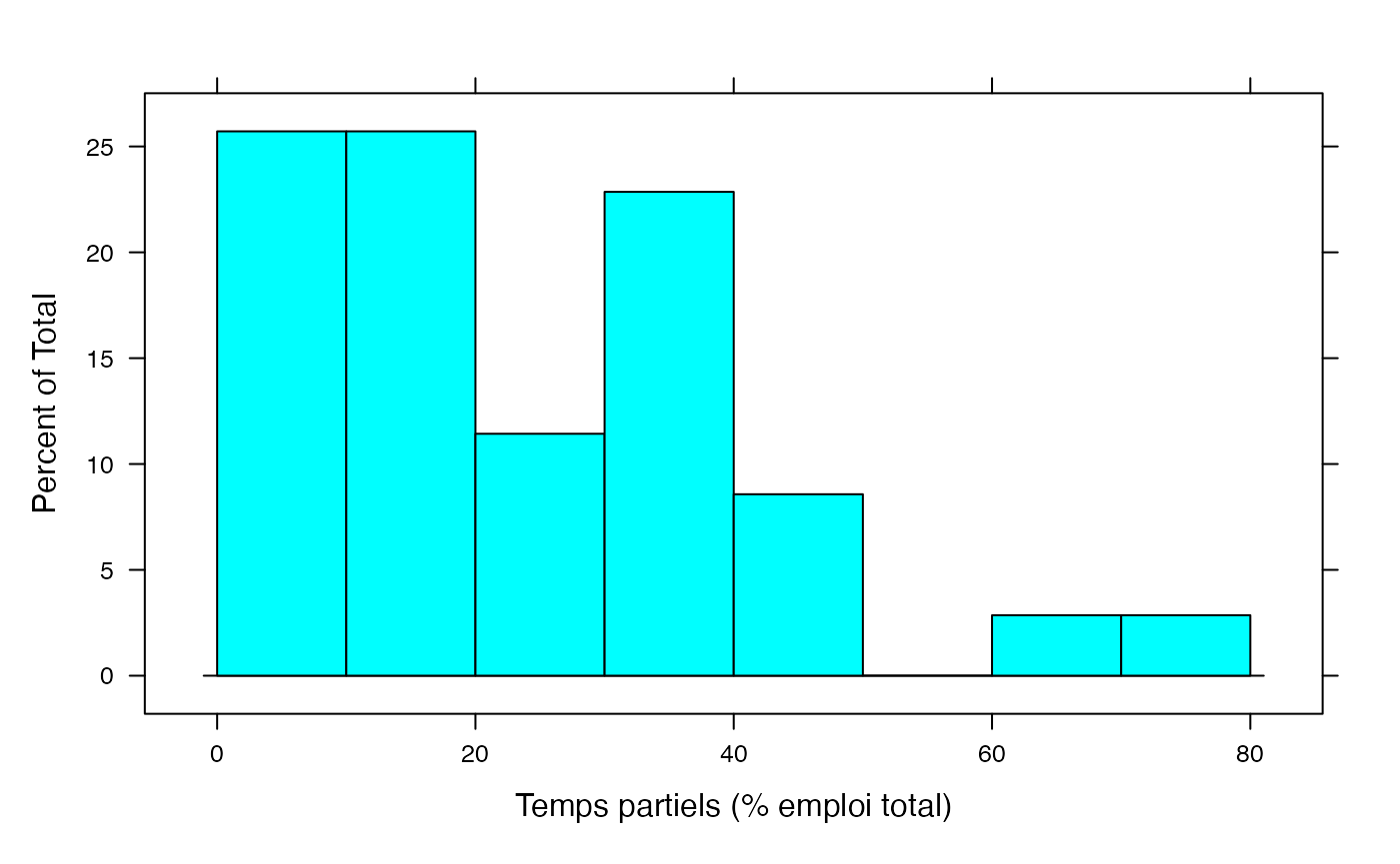
Les deux ensemble
par(mar = c(3, 3, 1, 1) + 0.1, mgp = c(2, 1, 0))
histogram(~Taux|Genre,xlab="Temps partiels (% emploi total)",data=Ensemble.df,breaks=c(0,10,20,30,40,50,60,70,80),layout=c(1,2))
Chemin <- "~/Documents/Recherche/DeBoeck/Graphes/Fichiers/"
colmodel="cmyk"
pdf(file = "HFfreqmargtempspartiel.pdf",
    width = 8, height = 7, onefile = TRUE, family = "Helvetica",
    title = "Probability or cumulative distribution graphs", paper = "special", colormodel = colmodel)
par(mar = c(3, 3, 1, 1) + 0.1, mgp = c(2, 1, 0))
histogram(~Taux|Genre,xlab="Temps partiels (% emploi total)",data=Ensemble.df,breaks=c(0,10,20,30,40,50,60,70,80),layout=c(1,2))
dev.off()
#> agg_png
#>       2
tfreqmargtempspartiel.pdf
par(mar = c(3, 3, 1, 1) + 0.1, mgp = c(2, 1, 0))
histogram(~Taux|Genre,xlab="Temps partiels (% emploi total)",data=Ensemble.df,breaks=c(0,10,20,30,40,50,60,70,80))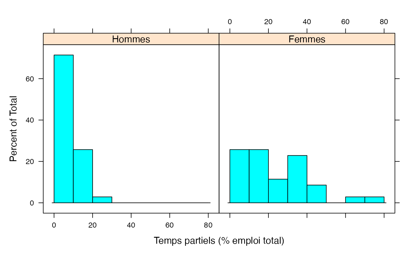
Chemin <- "~/Documents/Recherche/DeBoeck/Graphes/Fichiers/"
colmodel="cmyk"
pdf(file = "HFtfreqmargtempspartiel.pdf",
    width = 8, height = 7, onefile = TRUE, family = "Helvetica",
    title = "Probability or cumulative distribution graphs", paper = "special", colormodel = colmodel)
par(mar = c(3, 3, 1, 1) + 0.1, mgp = c(2, 1, 0))
histogram(~Taux|Genre,xlab="Temps partiels (% emploi total)",data=Ensemble.df,breaks=c(0,10,20,30,40,50,60,70,80))
dev.off()
#> agg_png
#>       2
freqcondX.pdf
#mp <- barplot(t(freqcondX),legend = rownames(freqcondX), ylim = c(0, 1)) # default
par(mar = c(3, 3, 1, 1) + 0.1, mgp = c(2, 1, 0))
mp <- barplot(t(freqcondX), beside=TRUE, legend = colnames(freqcondX), ylim = c(0, 1), args.legend=list(x="topleft",ncol=2,title="Femmes"),ylab="Pourcentage du total",xlab="Hommes") # default
#text(mp, t(freqcondX)+.05, format(freqcondX,digits=2), xpd = TRUE, col = "blue")
mtext(0:4*20,at=c(1+2*0:4),side=1)
mtext(0:4*20,at=c(10+2*0:4),side=1)
mtext(0:4*20,at=c(19+2*0:4),side=1)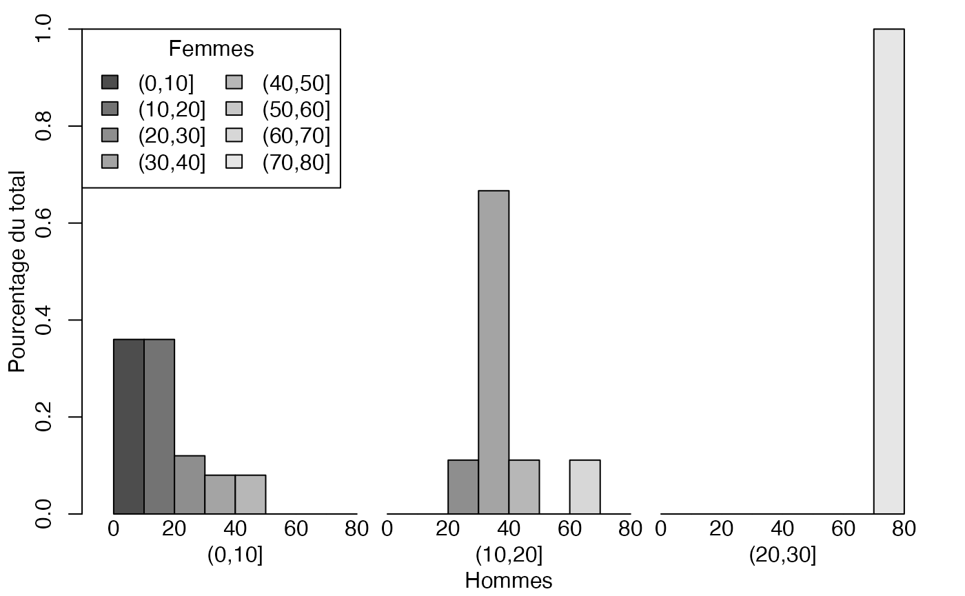
Chemin <- "~/Documents/Recherche/DeBoeck/Graphes/Fichiers/"
colmodel="cmyk"
pdf(file = "HFfreqcondX.pdf",
    width = 8, height = 7, onefile = TRUE, family = "Helvetica",
    title = "Probability or cumulative distribution graphs", paper = "special", colormodel = colmodel)
par(mar = c(3, 3, 1, 1) + 0.1, mgp = c(2, 1, 0))
mp <- barplot(t(freqcondX), beside=TRUE, legend = colnames(freqcondX), ylim = c(0, 1), args.legend=list(x="topleft",ncol=2,title="Femmes"),ylab="Pourcentage du total",xlab="Hommes") # default
#text(mp, t(freqcondX)+.05, format(freqcondX,digits=2), xpd = TRUE, col = "blue")
mtext(0:4*20,at=c(1+2*0:4),side=1)
mtext(0:4*20,at=c(10+2*0:4),side=1)
mtext(0:4*20,at=c(19+2*0:4),side=1)
dev.off()
#> agg_png
#>       2
freqcondY.pdf
#mp <- barplot(t(freqcondX),legend = rownames(freqcondX), ylim = c(0, 1)) # default
par(mar = c(3, 3, 1, 1) + 0.1, mgp = c(2, 1, 0))
mp <- barplot(freqcondY, beside=TRUE, legend = rownames(freqcondY), ylim = c(0, 1), args.legend=list(x="top",ncol=3,title="Hommes"),ylab="Pourcentage du total",xlab="Femmes") # default
#text(mp, t(freqcondX)+.05, format(freqcondX,digits=2), xpd = TRUE, col = "blue")
mtext(0:1*20,at=c(1+2*0:1),side=1)
mtext(0:1*20,at=c(5+2*0:1),side=1)
mtext(0:1*20,at=c(9+2*0:1),side=1)
mtext(0:1*20,at=c(13+2*0:1),side=1)
mtext(0:1*20,at=c(17+2*0:1),side=1)
mtext(0:1*20,at=c(21+2*0:1),side=1)
mtext(0:1*20,at=c(25+2*0:1),side=1)
mtext(0:1*20,at=c(29+2*0:1),side=1)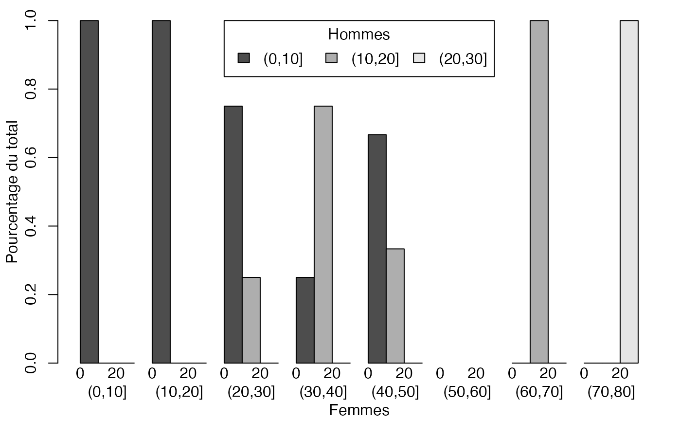
Chemin <- "~/Documents/Recherche/DeBoeck/Graphes/Fichiers/"
colmodel="cmyk"
pdf(file = "HFfreqcondY.pdf",
    width = 8, height = 7, onefile = TRUE, family = "Helvetica",
    title = "Probability or cumulative distribution graphs", paper = "special", colormodel = colmodel)
#mp <- barplot(t(freqcondX),legend = rownames(freqcondX), ylim = c(0, 1)) # default
par(mar = c(3, 3, 1, 1) + 0.1, mgp = c(2, 1, 0))
mp <- barplot(freqcondY, beside=TRUE, legend = rownames(freqcondY), ylim = c(0, 1), args.legend=list(x="top",ncol=3,title="Hommes"),ylab="Pourcentage du total",xlab="Femmes")  # default
#text(mp, t(freqcondX)+.05, format(freqcondX,digits=2), xpd = TRUE, col = "blue")
mtext(0:1*20,at=c(1+2*0:1),side=1)
mtext(0:1*20,at=c(5+2*0:1),side=1)
mtext(0:1*20,at=c(9+2*0:1),side=1)
mtext(0:1*20,at=c(13+2*0:1),side=1)
mtext(0:1*20,at=c(17+2*0:1),side=1)
mtext(0:1*20,at=c(21+2*0:1),side=1)
mtext(0:1*20,at=c(25+2*0:1),side=1)
mtext(0:1*20,at=c(29+2*0:1),side=1)
dev.off()
#> agg_png
#>       2
disptempspartiel.pdf
par(mar = c(3, 3, 1, 1) + 0.1, mgp = c(2, 1, 0))
plot(Europe$Partiel_H,Europe$Partiel_F,xlab="Hommes",ylab="Femmes",pch=19)
colmodel="cmyk"
Chemin <- "~/Documents/Recherche/DeBoeck/Graphes/Fichiers/"
colmodel="cmyk"
pdf(file = "HFdisptempspartiel.pdf",
    width = 8, height = 7, onefile = TRUE, family = "Helvetica",
    title = "Probability or cumulative distribution graphs", paper = "special", colormodel = colmodel)
par(mar = c(3, 3, 1, 1) + 0.1, mgp = c(2, 1, 0))
plot(Europe$Partiel_H,Europe$Partiel_F,xlab="Hommes",ylab="Femmes",pch=19)
dev.off()
#> agg_png
#>       2
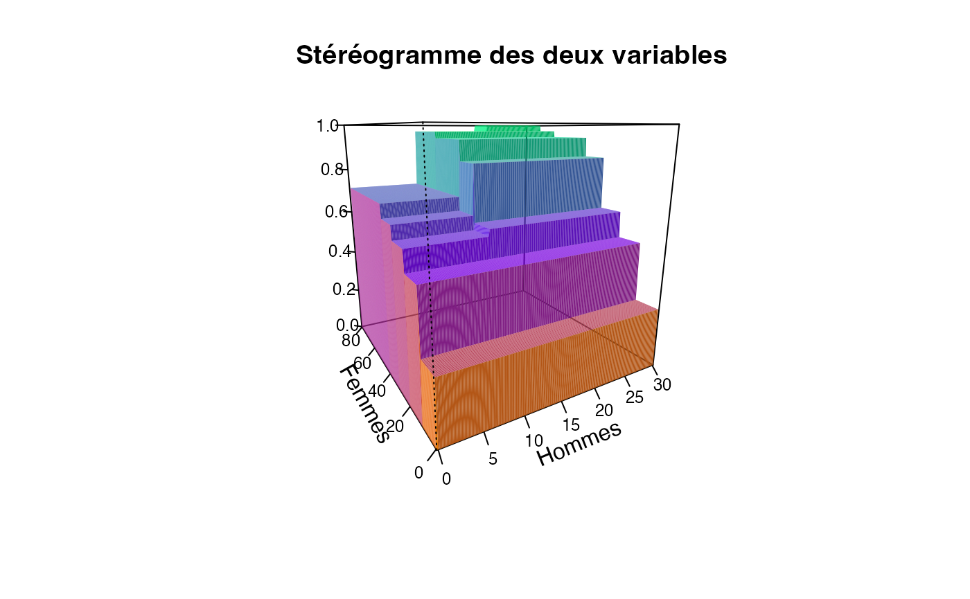
ff=table(cut(Europe$Partiel_H,c(0,10,20,30)),cut(Europe$Partiel_F,c(0,10,20,30,40,50,60,70,80)))/sum(table(cut(Europe$Partiel_H,c(0,10,20,30)),cut(Europe$Partiel_F,c(0,10,20,30,40,50,60,70,80))))
plotcdf3(c(0,10,20,30),c(0,10,20,30,40,50,60,70,80),f=ff,xaxe="Hommes",yaxe="Femmes",theme="0")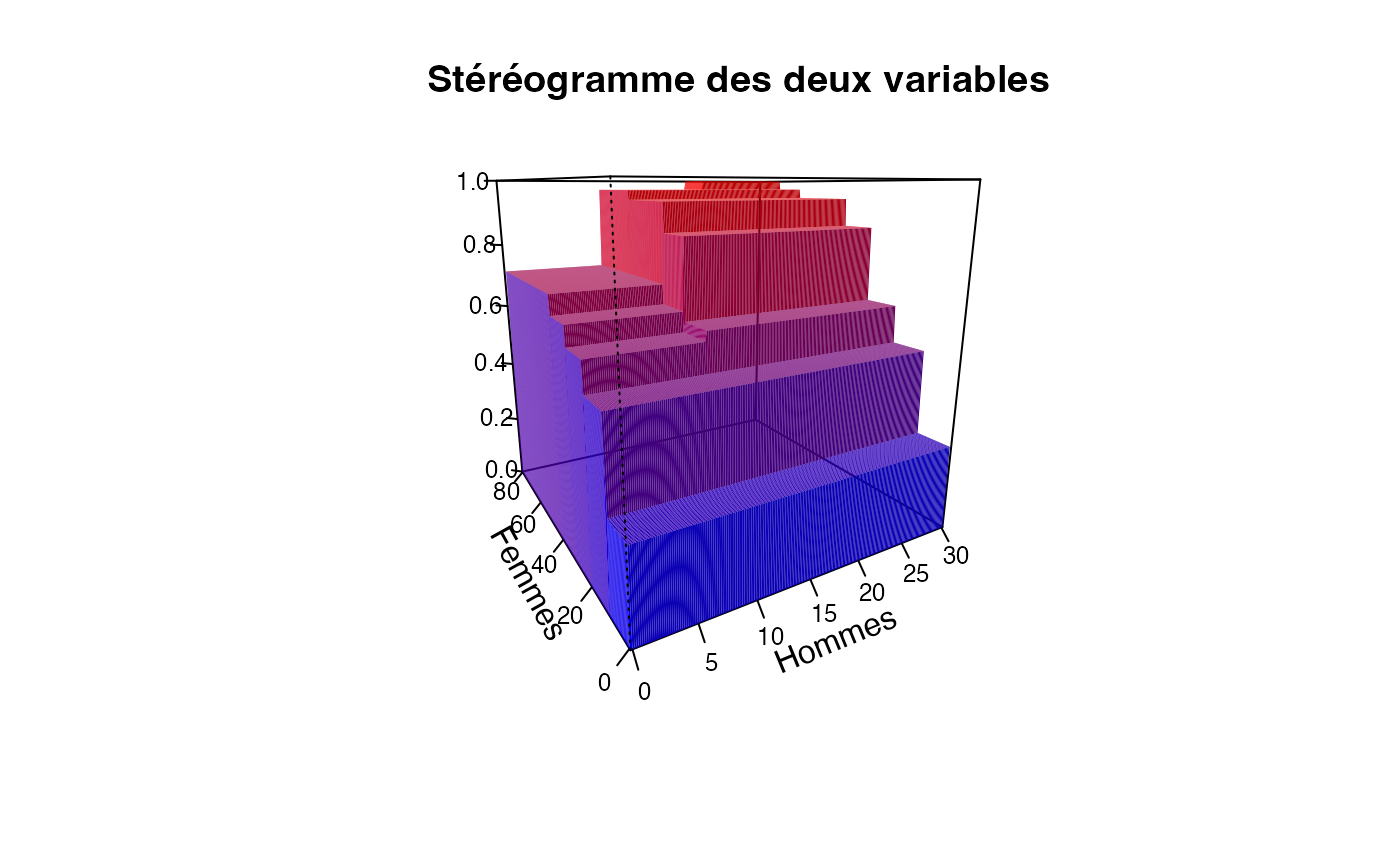

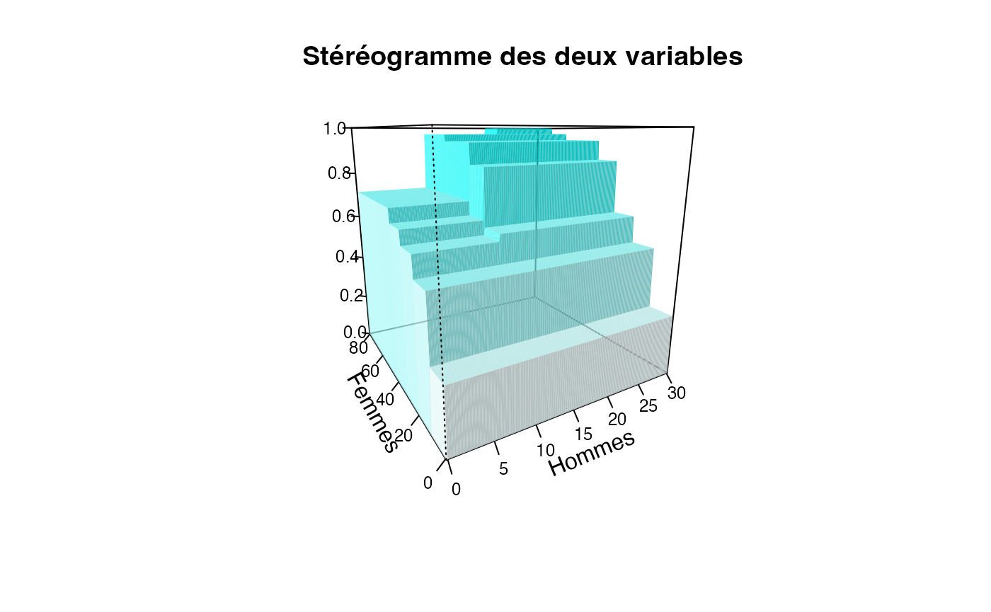
plotcdf3(c(0,10,20,30),c(0,10,20,30,40,50,60,70,80),f=ff,xaxe="Hommes",yaxe="Femmes",theme="cyan",border=TRUE)

Chemin <- "~/Documents/Recherche/DeBoeck/Graphes/Fichiers/"
colmodel="cmyk"
pdf(file = "HFstereotempspartiel.pdf",
    width = 8, height = 7, onefile = TRUE, family = "Helvetica",
    title = "Probability or cumulative distribution graphs", paper = "special", colormodel = colmodel)
par(mar = c(3, 3, 1, 1) + 0.1, mgp = c(2, 1, 0))
plotcdf3(c(0,10,20,30),c(0,10,20,30,40,50,60,70,80),f=ff,xaxe="Hommes",yaxe="Femmes",theme="cyan")
dev.off()
#> agg_png
#>       2
Provinces et territoires vs Sexe Canada (Quali-Quali)
data(ProtervsSexe_Canada)Distribution conditionnelle
ff=as.table(as.matrix(ProtervsSexe_Canada))/sum(as.table(as.matrix(ProtervsSexe_Canada)))

freqcondX <- prop.table(ff,1) #Y|X
freqcondY <- prop.table(ff,2) #Y|X
ensemble.df <- make.groups(freqcondX)
colnames(ensemble.df) <- c("Taux","ClasseX")
ensemble.df$ClasseX <- rep(colnames(ff),rep(length(rownames(ff)),length(colnames(ff))))
ensemble.df$ClasseY <- rep(rownames(ff),length(colnames(ff)))
ensemble.df
#>                  Taux ClasseX                   ClasseY
#> freqcondX1  0.4940692  Hommes   Terre-Neuve-et-Labrador
#> freqcondX2  0.4918277  Hommes     Île-du-Prince-Édouard
#> freqcondX3  0.4894997  Hommes           Nouvelle-Écosse
#> freqcondX4  0.4950210  Hommes         Nouveau-Brunswick
#> freqcondX5  0.4999521  Hommes                    Québec
#> freqcondX6  0.4940574  Hommes                   Ontario
#> freqcondX7  0.4992695  Hommes                  Manitoba
#> freqcondX8  0.5036927  Hommes              Saskatchewan
#> freqcondX9  0.5028255  Hommes                   Alberta
#> freqcondX10 0.4945358  Hommes      Colombie-Britannique
#> freqcondX11 0.5085846  Hommes                     Yukon
#> freqcondX12 0.5144040  Hommes Territoires du Nord-Ouest
#> freqcondX13 0.5118034  Hommes                   Nunavut
#> freqcondX14 0.5059308  Femmes   Terre-Neuve-et-Labrador
#> freqcondX15 0.5081723  Femmes     Île-du-Prince-Édouard
#> freqcondX16 0.5105003  Femmes           Nouvelle-Écosse
#> freqcondX17 0.5049790  Femmes         Nouveau-Brunswick
#> freqcondX18 0.5000479  Femmes                    Québec
#> freqcondX19 0.5059426  Femmes                   Ontario
#> freqcondX20 0.5007305  Femmes                  Manitoba
#> freqcondX21 0.4963073  Femmes              Saskatchewan
#> freqcondX22 0.4971745  Femmes                   Alberta
#> freqcondX23 0.5054642  Femmes      Colombie-Britannique
#> freqcondX24 0.4914154  Femmes                     Yukon
#> freqcondX25 0.4855960  Femmes Territoires du Nord-Ouest
#> freqcondX26 0.4881966  Femmes                   Nunavut
freqmargtempspartiel.pdf
Hommes<-ProtervsSexe_Canada$Hommes
Femmes<-ProtervsSexe_Canada$Femmes
Ensemble.df <- make.groups(Hommes,Femmes)
colnames(Ensemble.df) <- c("Taux","Genre")
Chemin <- "~/Documents/Recherche/DeBoeck/Graphes/Fichiers/"
colmodel="cmyk"
pdf(file = "CanPSmargcondX.pdf",
    width = 8, height = 7, onefile = TRUE, family = "Helvetica",
    title = "Probability or cumulative distribution graphs", paper = "special", colormodel = colmodel)
dotchart(rowSums(as.table(as.matrix(ProtervsSexe_Canada))),labels = rownames(ProtervsSexe_Canada))
dev.off()
#> agg_png
#>       2
Chemin <- "~/Documents/Recherche/DeBoeck/Graphes/Fichiers/"
colmodel="cmyk"
pdf(file = "CanPSmargcondY.pdf",
    width = 8, height = 7, onefile = TRUE, family = "Helvetica",
    title = "Probability or cumulative distribution graphs", paper = "special", colormodel = colmodel)
dotchart(colSums(as.table(as.matrix(ProtervsSexe_Canada))),labels = colnames(ProtervsSexe_Canada))
dev.off()
#> agg_png
#>       2
freqcondX.pdf
par(mar = c(7.5, 3, 1, 1) + 0.1, mgp = c(2, 1, 0))
mp <- barplot(t(freqcondX), beside=TRUE, legend = colnames(freqcondX), ylim = c(0, .65), las=2, srt=60, xaxt="n", args.legend=list(x="topleft",ncol=2),ylab="Pourcentage du total")
text(colMeans(mp), par("usr")[3], labels = rownames(freqcondX), srt = 60, adj = c(1.1,1.1), xpd = TRUE, cex=.8)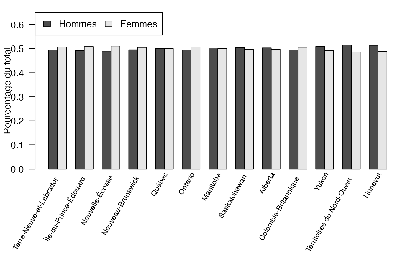
# default
Chemin <- "~/Documents/Recherche/DeBoeck/Graphes/Fichiers/"
colmodel="cmyk"
pdf(file = "CanPSfreqcondX.pdf",
    width = 8, height = 7, onefile = TRUE, family = "Helvetica",
    title = "Probability or cumulative distribution graphs", paper = "special", colormodel = colmodel)
par(mar = c(7.5, 3, 1, 1) + 0.1, mgp = c(2, 1, 0))
mp <- barplot(t(freqcondX), beside=TRUE, legend = colnames(freqcondX), ylim = c(0, .6), las=2, srt=60, xaxt="n", args.legend=list(x="topleft",ncol=2),ylab="Pourcentage du total")
text(colMeans(mp), par("usr")[3], labels = rownames(freqcondX), srt = 60, adj = c(1.1,1.1), xpd = TRUE, cex=.7)
# default
dev.off()
#> agg_png
#>       2
freqcondY.pdf
par(mar = c(3, 3, 1, 1) + 0.1, mgp = c(2, 1, 0))
mp <- barplot(freqcondX, beside=TRUE, legend = rownames(freqcondX), ylim = c(0, .85), las=2, srt=60, xaxt="n", args.legend=list(x="topleft",ncol=3,cex=.9),ylab="Pourcentage du total")
text(colMeans(mp), par("usr")[3], labels = colnames(freqcondX), srt = 60, adj = c(1.1,1.1), xpd = TRUE, cex=.8)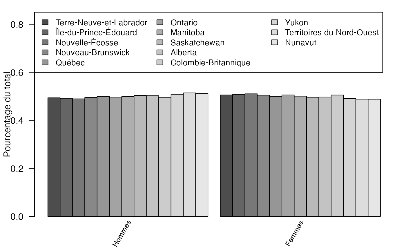
# default
Chemin <- "~/Documents/Recherche/DeBoeck/Graphes/Fichiers/"
colmodel="cmyk"
pdf(file = "CanPSfreqcondY.pdf",
    width = 8, height = 7, onefile = TRUE, family = "Helvetica",
    title = "Probability or cumulative distribution graphs", paper = "special", colormodel = colmodel)
par(mar = c(3, 3, 1, 1) + 0.1, mgp = c(2, 1, 0))
mp <- barplot(freqcondX, beside=TRUE, legend = rownames(freqcondX), ylim = c(0, .65), las=2, srt=60, xaxt="n", args.legend=list(x="topleft",ncol=3,cex=.9),ylab="Pourcentage du total")
text(colMeans(mp), par("usr")[3], labels = colnames(freqcondX), srt = 60, adj = c(1.1,1.1), xpd = TRUE, cex=.8)
# default
dev.off()
#> agg_png
#>       2
if(!("vcd" %in% installed.packages())){install.packages("vcd")}
library(vcd)
#> Loading required package: grid
mosaic(t(as.table(as.matrix(ProtervsSexe_Canada))), legend=TRUE,
   direction = "v", labeling= labeling_border(rot_labels = c(0,0,0,0),
   just_labels = c("center", "center", "center", "center"), varnames =  FALSE,offset_labels=c(0,0,0,4),gp_labels = gpar(fontsize = 6)))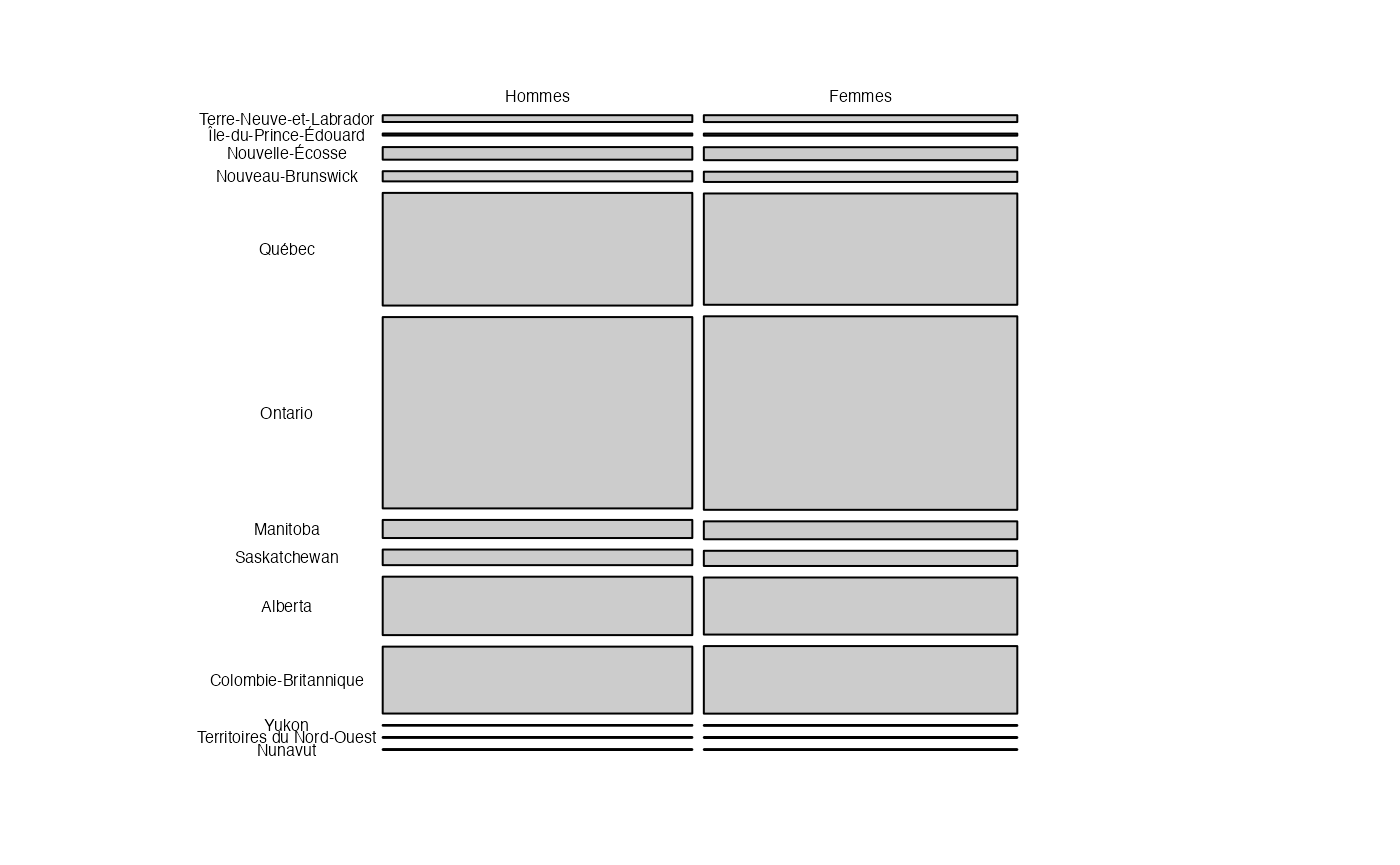
Chemin <- "~/Documents/Recherche/DeBoeck/Graphes/Fichiers/"
colmodel="cmyk"
pdf(file = "CanPSXY.pdf",
    width = 8, height = 7, onefile = TRUE, family = "Helvetica",
    title = "Probability or cumulative distribution graphs", paper = "special", colormodel = colmodel)
par(mar = c(3, 3, 1, 1) + 0.1, mgp = c(2, 1, 0))
mosaic(t(as.table(as.matrix(ProtervsSexe_Canada))), legend=TRUE,
   direction = "v", labeling= labeling_border(rot_labels = c(0,0,0,0),
   just_labels = c("center", "center", "center", "center"), varnames =  FALSE,offset_labels=c(0,0,0,4),gp_labels = gpar(fontsize = 6)))
dev.off()
#> agg_png
#>       2
Classe age vs Homme-Femme Canada (Quali-Quanti)
data(AgevsSexe_Canada_full)
AgevsSexe_Canada <- AgevsSexe_Canada_full[-nrow(AgevsSexe_Canada_full),]
AgevsSexe_Canada
#>              Hommes  Femmes
#> 0 à 4 ans    985452  936492
#> 5 à 9 ans   1045953  998650
#> 10 à 14 ans 1055313 1016787
#> 15 à 19 ans 1074091 1026774
#> 20 à 24 ans 1295347 1187455
#> 25 à 29 ans 1365844 1279396
#> 30 à 34 ans 1350274 1311449
#> 35 à 39 ans 1317432 1313248
#> 40 à 44 ans 1220034 1244213
#> 45 à 49 ans 1185148 1204968
#> 50 à 54 ans 1217865 1232050
#> 55 à 59 ans 1364677 1380219
#> 60 à 64 ans 1260206 1300035
#> 65 à 69 ans 1050581 1116694
#> 70 à 74 ans  854293  932329
#> 75 à 79 ans  569696  648607
#> 80 à 84 ans  359314  452056
#> 85 à 89 ans  208810  308900
#> 90 à 94 ans   84178  164415
#> 95 à 99 ans   18597   55879
Distribution conditionnelle
donnees = data.frame(
  Taux=c(AgevsSexe_Canada$Hommes,AgevsSexe_Canada$Femmes),
  Type=factor(c(rep("Hommes",nrow(AgevsSexe_Canada)),rep("Femmes",nrow(AgevsSexe_Canada)))))
tapply(donnees$Taux,donnees$Type,mean)
#>   Femmes   Hommes
#> 955530.8 944155.2
par(mar = c(2, 2, 1, 1) + 0.1, mgp = c(2, 1, 0))
pie(colSums(AgevsSexe_Canada),labels=levels(donnees$Type),col=c("white","#00FFFF","black","#00FFFF"),border=c("black","#00FFFF","black","#00FFFF"),density=25,cex=1.2)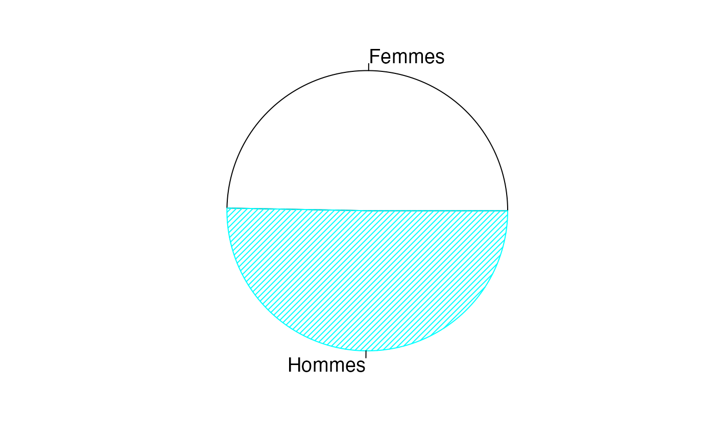
par(mar = c(2, 2, 1, 1) + 0.1, mgp = c(2, 1, 0))
dotplot(colSums(AgevsSexe_Canada),labels=levels(donnees$Type),col=c("black","black","black","black"),border=c("black","black","black","black"),density=25,cex=1.2, xlab = "Effectifs")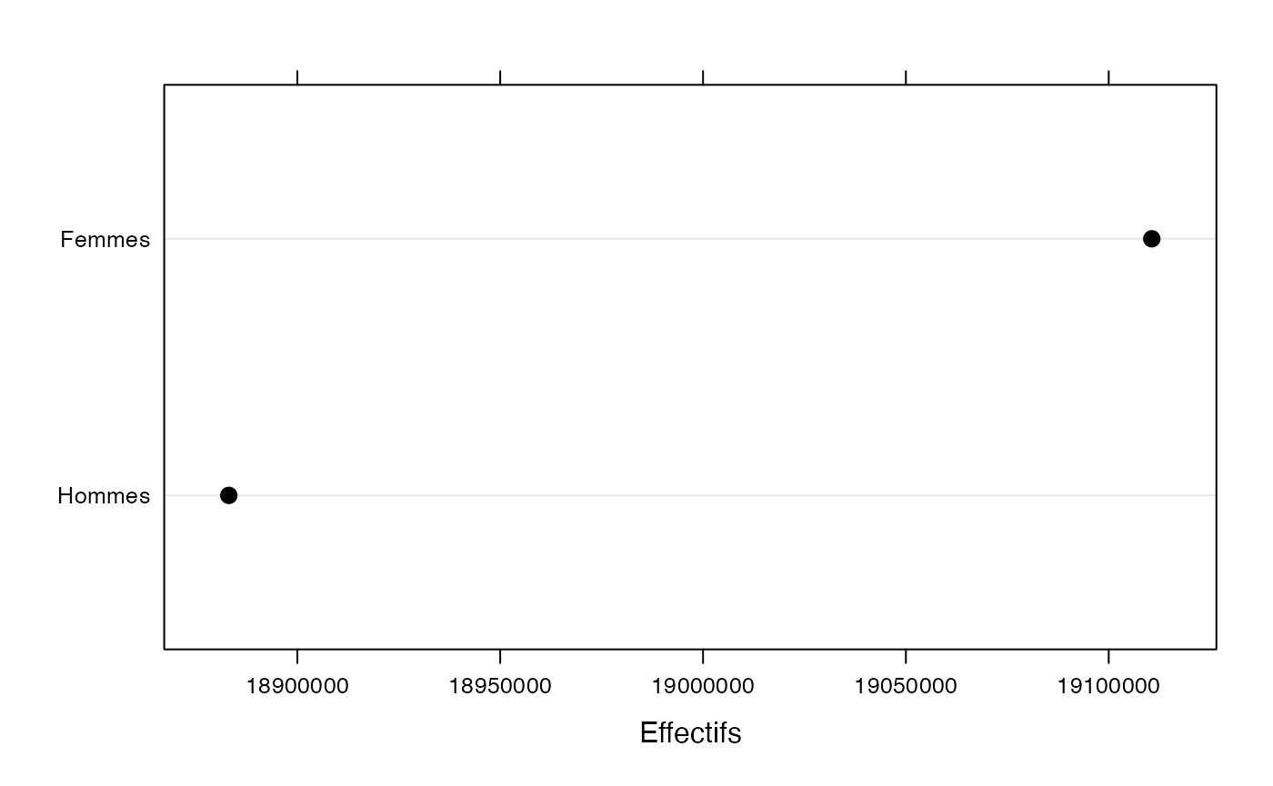
Chemin <- "~/Documents/Recherche/DeBoeck/Graphes/Fichiers/"
colmodel="cmyk"
pdf(file = "ASCpieqqualimarg.pdf",
    width = 8, height = 7, onefile = TRUE, family = "Helvetica",
    title = "Probability or cumulative distribution graphs", paper = "special", colormodel = colmodel)
par(mar = c(2, 2, 1, 1) + 0.1, mgp = c(2, 1, 0))
pie(colSums(AgevsSexe_Canada),labels=levels(donnees$Type),col=c("white","#00FFFF","black","#00FFFF"),border=c("black","#00FFFF","black","#00FFFF"),density=25,cex=1.2)
dev.off()
#> agg_png
#>       2

pdf(file = "ASCqqualimarg.pdf",
    width = 8, height = 7, onefile = TRUE, family = "Helvetica",
    title = "Probability or cumulative distribution graphs", paper = "special", colormodel = colmodel)
par(mar = c(2, 2, 1, 1) + 0.1, mgp = c(2, 1, 0))
dotplot(colSums(AgevsSexe_Canada),labels=levels(donnees$Type),col=c("black","black","black","black"),border=c("black","black","black","black"),density=25,cex=1.2, xlab = "Effectifs")
dev.off()
#> agg_png
#>       2
sumdat<-data.frame(Âge=rep((0:19)*5+2.5,rowSums(AgevsSexe_Canada)))
histogram(~Âge,data=sumdat,breaks=(0:20)*5)
Chemin <- "~/Documents/Recherche/DeBoeck/Graphes/Fichiers/"
colmodel="cmyk"
pdf(file = "ASCqquantimarg.pdf",
    width = 8, height = 7, onefile = TRUE, family = "Helvetica",
    title = "Probability or cumulative distribution graphs", paper = "special", colormodel = colmodel)
par(mar = c(2, 2, 1, 1) + 0.1, mgp = c(2, 1, 0))
histogram(~Âge,data=sumdat,breaks=(0:20)*5)
dev.off()
#> agg_png
#>       2
fulldat<-data.frame(Âge=c(rep((0:19)*5+2.5,AgevsSexe_Canada[,1]),
                          rep((0:19)*5+2.5,AgevsSexe_Canada[,2])
                          ),
                  Type=factor(c(rep("Homme",sum(AgevsSexe_Canada[,1])),rep("Femme",sum(AgevsSexe_Canada[,2]))))
)
#summary(fulldat)
histogram(~Âge|Type,data=fulldat,breaks=(0:20)*5)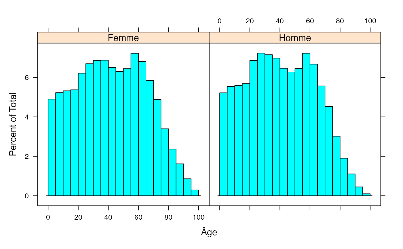
Chemin <- "~/Documents/Recherche/DeBoeck/Graphes/Fichiers/"
colmodel="cmyk"
pdf(file = "ASCqquanticond.pdf",
    width = 8, height = 7, onefile = TRUE, family = "Helvetica",
    title = "Probability or cumulative distribution graphs", paper = "special", colormodel = colmodel)
par(mar = c(2, 2, 1, 1) + 0.1, mgp = c(2, 1, 0))
histogram(~Âge|Type,data=fulldat,breaks=(0:20)*5)
dev.off()
#> agg_png
#>       2
TauxQuali <- cut(fulldat$Âge,breaks=(0:20)*5)
#split(fulldat$Type,TauxQuali)
sapply(split(fulldat$Type,TauxQuali),table)
#>        (0,5]  (5,10] (10,15] (15,20] (20,25] (25,30] (30,35] (35,40] (40,45]
#> Femme 936492  998650 1016787 1026774 1187455 1279396 1311449 1313248 1244213
#> Homme 985452 1045953 1055313 1074091 1295347 1365844 1350274 1317432 1220034
#>       (45,50] (50,55] (55,60] (60,65] (65,70] (70,75] (75,80] (80,85] (85,90]
#> Femme 1204968 1232050 1380219 1300035 1116694  932329  648607  452056  308900
#> Homme 1185148 1217865 1364677 1260206 1050581  854293  569696  359314  208810
#>       (90,95] (95,100]
#> Femme  164415    55879
#> Homme   84178    18597

regroup <- sapply(split(fulldat$Type,TauxQuali),table)
par(mar = c(3, 3, 1, 1) + 0.1, mgp = c(2, 1, 0))
barplot(regroup,beside=TRUE, legend=levels(donnees$Type), args.legend=list(x="topright", ncol=1),las=2)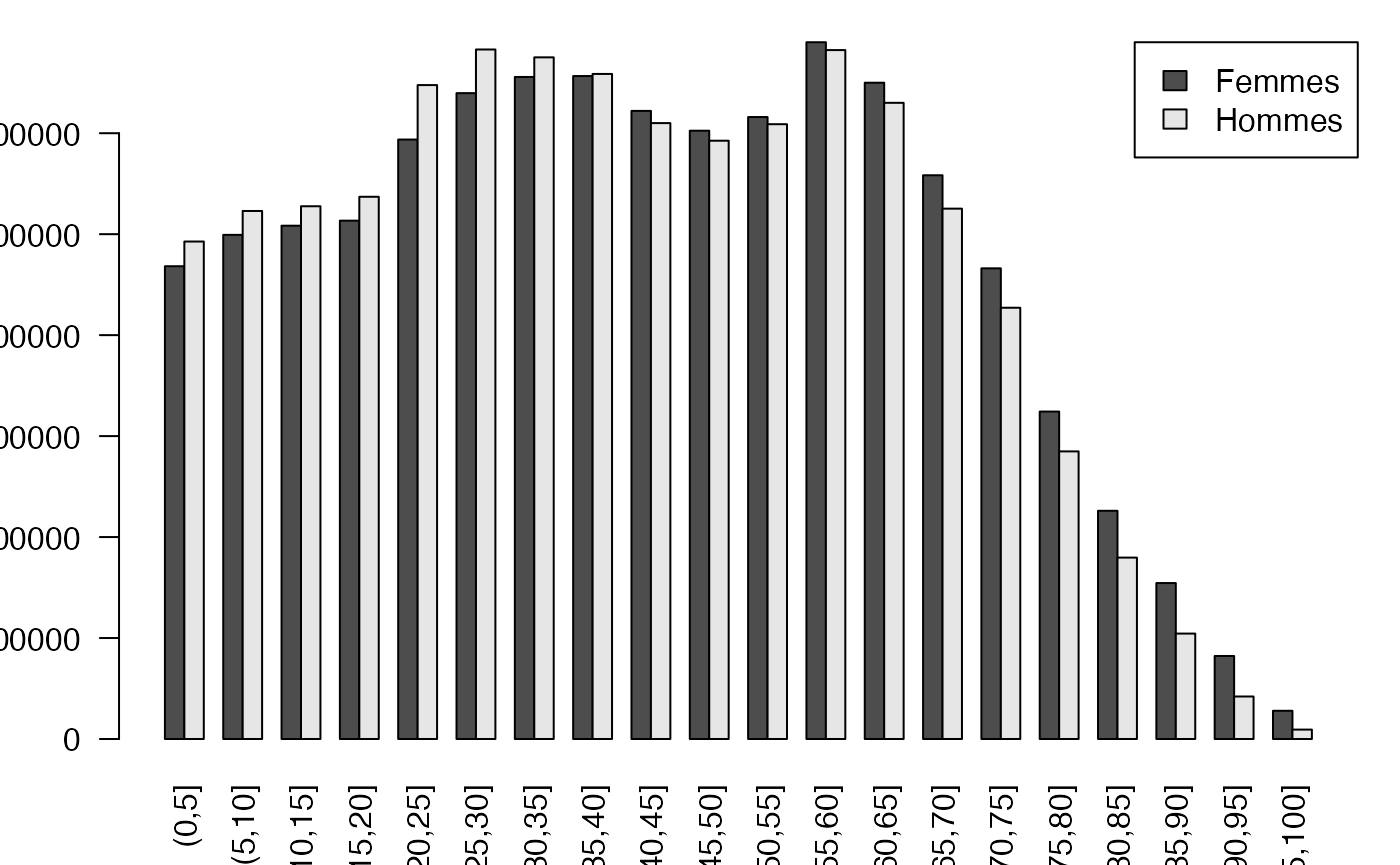
Chemin <- "~/Documents/Recherche/DeBoeck/Graphes/Fichiers/"
colmodel="cmyk"
pdf(file = "ASCqqualicond.pdf",
    width = 8, height = 7, onefile = TRUE, family = "Helvetica",
    title = "Probability or cumulative distribution graphs", paper = "special", colormodel = colmodel)
par(mar = c(4.5, 4.5, 1, 1) + 0.1, mgp = c(2, 1, 0))
barplot(regroup,beside=TRUE, legend=levels(donnees$Type), args.legend=list(x="topright", ncol=1),las=2)
dev.off()
#> agg_png
#>       2
Classe age vs Provinces et territoires Canada (Quali-Quanti)
data(AgevsProter_Canada_full)
AgevsProter_Canada <- AgevsProter_Canada_full[-nrow(AgevsProter_Canada_full),]
AgevsProter_Canada
#>             Terre.Neuve.et.Labrador Île.du.Prince.Édouard Nouvelle.Écosse
#> 0 à 4 ans                     20402                  7199           42443
#> 5 à 9 ans                     23376                  8248           46177
#> 10 à 14 ans                   26186                  8966           48170
#> 15 à 19 ans                   26994                  9340           50776
#> 20 à 24 ans                   28910                 11577           61556
#> 25 à 29 ans                   28076                 10321           63359
#> 30 à 34 ans                   28942                  9212           61264
#> 35 à 39 ans                   30151                  9314           58683
#> 40 à 44 ans                   31426                  9586           56907
#> 45 à 49 ans                   35754                 10231           61194
#> 50 à 54 ans                   40214                 10319           65276
#> 55 à 59 ans                   43105                 12005           78780
#> 60 à 64 ans                   42339                 11350           75941
#> 65 à 69 ans                   39718                 10116           66676
#> 70 à 74 ans                   33179                  9106           57399
#> 75 à 79 ans                   20458                  5589           37734
#> 80 à 84 ans                   12617                  3641           24225
#> 85 à 89 ans                    6662                  2244           14184
#> 90 à 94 ans                    2715                   935            6318
#> 95 à 99 ans                     751                   281            1930
#>             Nouveau.Brunswick Québec Ontario Manitoba Saskatchewan Alberta
#> 0 à 4 ans               33582 430250  723016    85220        75200  269163
#> 5 à 9 ans               38199 465890  762654    89507        78696  277785
#> 10 à 14 ans             40354 457420  792947    86583        76730  276328
#> 15 à 19 ans             40662 426496  852405    85808        71304  256742
#> 20 à 24 ans             43490 499370 1039661    96636        75402  277328
#> 25 à 29 ans             43981 564669 1077433    97157        77488  314507
#> 30 à 34 ans             44703 548066 1041952    98789        85751  356226
#> 35 à 39 ans             46655 578273  992844    95203        86664  359301
#> 40 à 44 ans             48179 581724  921378    86739        76067  319889
#> 45 à 49 ans             51551 527233  932058    82541        67397  288546
#> 50 à 54 ans             54044 546847  968546    80302        65716  266489
#> 55 à 59 ans             63300 637724 1073519    89949        77024  284259
#> 60 à 64 ans             61514 619126  961243    83163        74222  264339
#> 65 à 69 ans             55477 529279  803962    70981        62071  210073
#> 70 à 74 ans             46962 440008  673546    57001        46528  157657
#> 75 à 79 ans             30462 313752  461015    38329        31910  102977
#> 80 à 84 ans             19475 198497  319548    25922        22791   68565
#> 85 à 89 ans             11705 128147  204227    16952        15931   44033
#> 90 à 94 ans              5213  60879   98638     8968         8492   20921
#> 95 à 99 ans              1704  18086   29527     3010         2773    5746
#>             Colombie.Britannique Yukon TerritoiresduNord.Ouest Nunavut
#> 0 à 4 ans                 225897  2413                    2963    4196
#> 5 à 9 ans                 244206  2508                    3081    4276
#> 10 à 14 ans               249173  2246                    3010    3987
#> 15 à 19 ans               272195  2067                    2793    3283
#> 20 à 24 ans               340325  2346                    3028    3173
#> 25 à 29 ans               358457  2828                    3688    3276
#> 30 à 34 ans               376466  3468                    3705    3179
#> 35 à 39 ans               363871  3549                    3405    2767
#> 40 à 44 ans               323620  3050                    3348    2334
#> 45 à 49 ans               325674  2864                    2919    2154
#> 50 à 54 ans               343894  2753                    3238    2277
#> 55 à 59 ans               376848  3233                    3389    1761
#> 60 à 64 ans               360150  3116                    2619    1119
#> 65 à 69 ans               314021  2385                    1818     698
#> 70 à 74 ans               262197  1532                    1048     459
#> 75 à 79 ans               174377   862                     603     235
#> 80 à 84 ans               115218   464                     293     114
#> 85 à 89 ans                73205   246                     133      41
#> 90 à 94 ans                35355    84                      57      18
#> 95 à 99 ans                10613    31                      21       3
Distribution conditionnelle
donnees = data.frame(
  Âge=c(AgevsProter_Canada$Terre.Neuve.et.Labrador,AgevsProter_Canada$Île.du.Prince.Édouard,AgevsProter_Canada$Nouvelle.Écosse,AgevsProter_Canada$Nouveau.Brunswick,AgevsProter_Canada$Québec,AgevsProter_Canada$Ontario,AgevsProter_Canada$Manitoba,AgevsProter_Canada$Saskatchewan,AgevsProter_Canada$Alberta,AgevsProter_Canada$Colombie.Britannique,AgevsProter_Canada$Yukon,AgevsProter_Canada$TerritoiresduNord.Ouest,AgevsProter_Canada$Nunavut),
  Type=factor(
    c(rep("Terre Neuve et Labrador",nrow(AgevsProter_Canada)),
      rep("Île du Prince Édouard",nrow(AgevsProter_Canada)),
      rep("Nouvelle Écosse",nrow(AgevsProter_Canada)),
      rep("Nouveau Brunswick",nrow(AgevsProter_Canada)),
      rep("Québec",nrow(AgevsProter_Canada)),
      rep("Ontario",nrow(AgevsProter_Canada)),
      rep("Manitoba",nrow(AgevsProter_Canada)),
      rep("Saskatchewan",nrow(AgevsProter_Canada)),
      rep("Alberta",nrow(AgevsProter_Canada)),
      rep("Colombie Britannique",nrow(AgevsProter_Canada)),
      rep("Yukon",nrow(AgevsProter_Canada)),
      rep("Territoires du Nord Ouest",nrow(AgevsProter_Canada)),
      rep("Nunavut",nrow(AgevsProter_Canada))
      )))
tapply(donnees$Âge,donnees$Type,mean)
#>                   Alberta      Colombie Britannique     Île du Prince Édouard
#>                 221043.70                 257288.10                   7979.00
#>                  Manitoba         Nouveau Brunswick           Nouvelle Écosse
#>                  68938.00                  39060.60                  48949.60
#>                   Nunavut                   Ontario                    Québec
#>                   1967.50                 736505.95                 428586.80
#>              Saskatchewan   Terre Neuve et Labrador Territoires du Nord Ouest
#>                  58907.85                  26098.75                   2257.95
#>                     Yukon
#>                   2102.25
nameXlit <- c("Terre Neuve et Labrador",
  "Île du Prince Édouard",
  "Nouvelle Écosse",
  "Nouveau Brunswick",
  "Québec",
  "Ontario",
  "Manitoba",
  "\nSaskatchewan",
  "Alberta",
  "Colombie Britannique",
  "\nYukon",
  "\n\n\nTerritoires du Nord Ouest",
  "Nunavut")
par(mar = c(2, 2, 1, 1) + 0.1, mgp = c(2, 1, 0))
pie(colSums(AgevsProter_Canada),labels=nameXlit,col=c("white","#00FFFF","black","#00FFFF"),border=c("black","#00FFFF","black","#00FFFF"),density=25,cex=.6)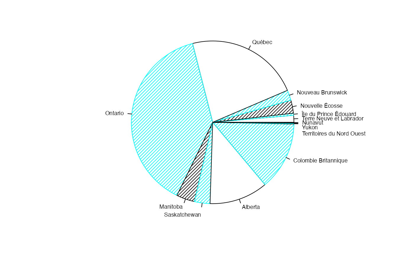
par(mar = c(2, 2, 1, 1) + 0.1, mgp = c(2, 1, 0))
dotplot(colSums(AgevsProter_Canada),labels=levels(donnees$Type),col=c("black","black","black","black"),border=c("black","black","black","black"),density=25,cex=1.2)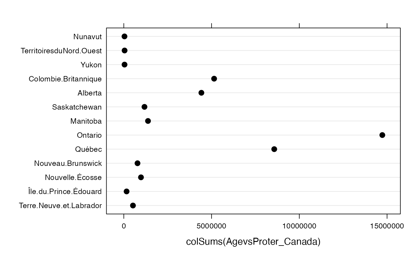
Chemin <- "~/Documents/Recherche/DeBoeck/Graphes/Fichiers/"
colmodel="cmyk"
pdf(file = "ATPCpieqqualimarg.pdf",
    width = 8, height = 7, onefile = TRUE, family = "Helvetica",
    title = "Probability or cumulative distribution graphs", paper = "special", colormodel = colmodel)
par(mar = c(2, 2, 1, 1) + 0.1, mgp = c(2, 1, 0))
pie(colSums(AgevsProter_Canada),labels=nameXlit,col=c("white","#00FFFF","black","#00FFFF"),border=c("black","#00FFFF","black","#00FFFF"),density=25,cex=.6)
dev.off()
#> agg_png
#>       2

pdf(file = "ATPCqqualimarg.pdf",
    width = 8, height = 7, onefile = TRUE, family = "Helvetica",
    title = "Probability or cumulative distribution graphs", paper = "special", colormodel = colmodel)
par(mar = c(2, 2, 1, 1) + 0.1, mgp = c(2, 1, 0))
dotplot(colSums(AgevsProter_Canada),labels=levels(donnees$Type),col=c("black","black","black","black"),border=c("black","black","black","black"),density=25,cex=1.2,xlab = "Effectifs")
dev.off()
#> agg_png
#>       2
sumdat<-data.frame(Âge=rep((0:19)*5+2.5,rowSums(AgevsProter_Canada)))
histogram(~Âge,data=sumdat,breaks=(0:20)*5)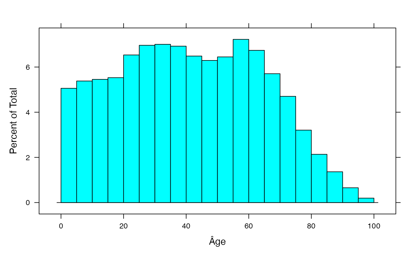
Chemin <- "~/Documents/Recherche/DeBoeck/Graphes/Fichiers/"
colmodel="cmyk"
pdf(file = "ATPCqquantimarg.pdf",
    width = 8, height = 7, onefile = TRUE, family = "Helvetica",
    title = "Probability or cumulative distribution graphs", paper = "special", colormodel = colmodel)
par(mar = c(2, 2, 1, 1) + 0.1, mgp = c(2, 1, 0))
histogram(~Âge,data=sumdat,breaks=(0:20)*5)
dev.off()
#> agg_png
#>       2
fulldat<-data.frame(Âge=c(rep((0:19)*5+2.5,AgevsProter_Canada[,1]),
                          rep((0:19)*5+2.5,AgevsProter_Canada[,2]),
                          rep((0:19)*5+2.5,AgevsProter_Canada[,3]),
                          rep((0:19)*5+2.5,AgevsProter_Canada[,4]),
                          rep((0:19)*5+2.5,AgevsProter_Canada[,5]),
                          rep((0:19)*5+2.5,AgevsProter_Canada[,6]),
                          rep((0:19)*5+2.5,AgevsProter_Canada[,7]),
                          rep((0:19)*5+2.5,AgevsProter_Canada[,8]),
                          rep((0:19)*5+2.5,AgevsProter_Canada[,9]),
                          rep((0:19)*5+2.5,AgevsProter_Canada[,10]),
                          rep((0:19)*5+2.5,AgevsProter_Canada[,11]),
                          rep((0:19)*5+2.5,AgevsProter_Canada[,12]),
                          rep((0:19)*5+2.5,AgevsProter_Canada[,13])
                          ),
                  Type=factor(
    c(rep("T. Neuve et Lab.",sum(AgevsProter_Canada[,1])),
      rep("Île Pr Édouard",sum(AgevsProter_Canada[,2])),
      rep("Nouv. Écosse",sum(AgevsProter_Canada[,3])),
      rep("Nouv. Brunswick",sum(AgevsProter_Canada[,4])),
      rep("Québec",sum(AgevsProter_Canada[,5])),
      rep("Ontario",sum(AgevsProter_Canada[,6])),
      rep("Manitoba",sum(AgevsProter_Canada[,7])),
      rep("Saskatch.",sum(AgevsProter_Canada[,8])),
      rep("Alberta",sum(AgevsProter_Canada[,9])),
      rep("Col. Brit.",sum(AgevsProter_Canada[,10])),
      rep("Yukon",sum(AgevsProter_Canada[,11])),
      rep("T. du Nord Ouest",sum(AgevsProter_Canada[,12])),
      rep("Nunavut",sum(AgevsProter_Canada[,13]))
      ))
)
#summary(fulldat)
histogram(~Âge|Type,data=fulldat,breaks=(0:20)*5)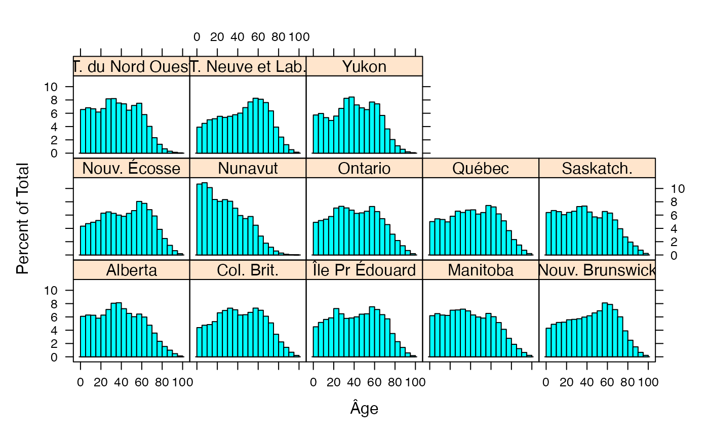
Chemin <- "~/Documents/Recherche/DeBoeck/Graphes/Fichiers/"
colmodel="cmyk"
pdf(file = "ATPCqquanticond.pdf",
    width = 8, height = 7, onefile = TRUE, family = "Helvetica",
    title = "Probability or cumulative distribution graphs", paper = "special", colormodel = colmodel)
par(mar = c(2, 2, 1, 1) + 0.1, mgp = c(2, 1, 0))
histogram(~Âge|Type,data=fulldat,breaks=(0:20)*5)
dev.off()
#> agg_png
#>       2
TauxQuali <- cut(fulldat$Âge,breaks=(0:20)*5)
#split(fulldat$Type,TauxQuali)
sapply(split(fulldat$Type,TauxQuali),table)
#>                   (0,5] (5,10] (10,15] (15,20] (20,25] (25,30] (30,35] (35,40]
#> Alberta          269163 277785  276328  256742  277328  314507  356226  359301
#> Col. Brit.       225897 244206  249173  272195  340325  358457  376466  363871
#> Île Pr Édouard     7199   8248    8966    9340   11577   10321    9212    9314
#> Manitoba          85220  89507   86583   85808   96636   97157   98789   95203
#> Nouv. Brunswick   33582  38199   40354   40662   43490   43981   44703   46655
#> Nouv. Écosse      42443  46177   48170   50776   61556   63359   61264   58683
#> Nunavut            4196   4276    3987    3283    3173    3276    3179    2767
#> Ontario          723016 762654  792947  852405 1039661 1077433 1041952  992844
#> Québec           430250 465890  457420  426496  499370  564669  548066  578273
#> Saskatch.         75200  78696   76730   71304   75402   77488   85751   86664
#> T. du Nord Ouest   2963   3081    3010    2793    3028    3688    3705    3405
#> T. Neuve et Lab.  20402  23376   26186   26994   28910   28076   28942   30151
#> Yukon              2413   2508    2246    2067    2346    2828    3468    3549
#>                  (40,45] (45,50] (50,55] (55,60] (60,65] (65,70] (70,75]
#> Alberta           319889  288546  266489  284259  264339  210073  157657
#> Col. Brit.        323620  325674  343894  376848  360150  314021  262197
#> Île Pr Édouard      9586   10231   10319   12005   11350   10116    9106
#> Manitoba           86739   82541   80302   89949   83163   70981   57001
#> Nouv. Brunswick    48179   51551   54044   63300   61514   55477   46962
#> Nouv. Écosse       56907   61194   65276   78780   75941   66676   57399
#> Nunavut             2334    2154    2277    1761    1119     698     459
#> Ontario           921378  932058  968546 1073519  961243  803962  673546
#> Québec            581724  527233  546847  637724  619126  529279  440008
#> Saskatch.          76067   67397   65716   77024   74222   62071   46528
#> T. du Nord Ouest    3348    2919    3238    3389    2619    1818    1048
#> T. Neuve et Lab.   31426   35754   40214   43105   42339   39718   33179
#> Yukon               3050    2864    2753    3233    3116    2385    1532
#>                  (75,80] (80,85] (85,90] (90,95] (95,100]
#> Alberta           102977   68565   44033   20921     5746
#> Col. Brit.        174377  115218   73205   35355    10613
#> Île Pr Édouard      5589    3641    2244     935      281
#> Manitoba           38329   25922   16952    8968     3010
#> Nouv. Brunswick    30462   19475   11705    5213     1704
#> Nouv. Écosse       37734   24225   14184    6318     1930
#> Nunavut              235     114      41      18        3
#> Ontario           461015  319548  204227   98638    29527
#> Québec            313752  198497  128147   60879    18086
#> Saskatch.          31910   22791   15931    8492     2773
#> T. du Nord Ouest     603     293     133      57       21
#> T. Neuve et Lab.   20458   12617    6662    2715      751
#> Yukon                862     464     246      84       31

regroup <- sapply(split(fulldat$Type,TauxQuali),table)
par(mar = c(4.5, 4, 1, 1) + 0.1, mgp = c(2, 1, 0))
barplot(regroup,beside=TRUE, legend=levels(donnees$Type), args.legend=list(x="topright", ncol=4,cex=.6),las=2,ylim=c(0,1.4e6))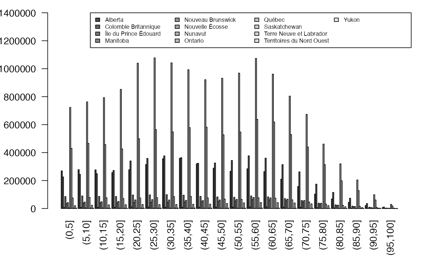
Chemin <- "~/Documents/Recherche/DeBoeck/Graphes/Fichiers/"
colmodel="cmyk"
pdf(file = "ATPCqqualicond.pdf",
    width = 8, height = 7, onefile = TRUE, family = "Helvetica",
    title = "Probability or cumulative distribution graphs", paper = "special", colormodel = colmodel)
par(mar = c(4.5, 4.5, 1, 1) + 0.1, mgp = c(2, 1, 0))
barplot(regroup,beside=TRUE, legend=levels(donnees$Type), args.legend=list(x="topright", ncol=4,cex=.6),las=2,ylim=c(0,1.25e6))
dev.off()
#> agg_png
#>       2
Bonus Europe Siège-Voix
data(Sieges_Voix)

str(Sieges_Voix)
#> 'data.frame':    27 obs. of  4 variables:
#>  $ Etats.Membres      : chr  "Allemagne" "Autriche" "Belgique" "Bulgarie" ...
#>  $ Date.entrée        : int  1957 1995 1957 2007 2004 1973 1986 2004 1995 1957 ...
#>  $ Sièges.au.parlement: int  99 18 24 0 6 14 54 6 14 78 ...
#>  $ Voix.au.conseil    : int  29 10 12 0 4 7 27 4 7 29 ...
summary(Sieges_Voix)
#>  Etats.Membres       Date.entrée   Sièges.au.parlement Voix.au.conseil
#>  Length:27          Min.   :1957   Min.   : 0.00       Min.   : 0.00
#>  Class :character   1st Qu.:1973   1st Qu.: 8.00       1st Qu.: 4.00
#>  Mode  :character   Median :1995   Median :18.00       Median :10.00
#>                     Mean   :1987   Mean   :27.11       Mean   :11.89
#>                     3rd Qu.:2004   3rd Qu.:25.50       3rd Qu.:12.50
#>                     Max.   :2007   Max.   :99.00       Max.   :29.00
NameX <- Sieges_Voix$Etats.Membres
NombreSieges <- Sieges_Voix$Sièges.au.parlement
NombreVoix <- Sieges_Voix$Voix.au.conseil
NameXX <- names(table(Sieges_Voix$Date.entrée))
NombreAnnees <- as.vector(table(Sieges_Voix$Date.entrée))

names(NombreSieges) <- NameX
NombreSieges
#>          Allemagne           Autriche           Belgique           Bulgarie
#>                 99                 18                 24                  0
#>             Chypre           Danemark            Espagne            Estonie
#>                  6                 14                 54                  6
#>           Finlande             France              Grèce            Hongrie
#>                 14                 78                 24                 24
#>            Irlande             Italie           Lettonie           Lituanie
#>                 13                 78                  9                 13
#>         Luxembourg              Malte           Pays-Bas            Pologne
#>                  6                  5                 27                 54
#>           Portugal République Tchèque           Roumanie        Royaume-Uni
#>                 24                 24                  0                 78
#>          Slovaquie           Slovénie              Suède
#>                 14                  7                 19
Année <- Sieges_Voix$Date.entrée
Pays <- NameX
Europ <- rbind(NombreSieges,NombreVoix)
colnames(Europ) <- Pays
margin.table(Europ)
#> [1] 1053
margin.table(Europ,1)
#> NombreSieges   NombreVoix
#>          732          321
margin.table(Europ,2)
#>          Allemagne           Autriche           Belgique           Bulgarie
#>                128                 28                 36                  0
#>             Chypre           Danemark            Espagne            Estonie
#>                 10                 21                 81                 10
#>           Finlande             France              Grèce            Hongrie
#>                 21                107                 36                 36
#>            Irlande             Italie           Lettonie           Lituanie
#>                 20                107                 13                 20
#>         Luxembourg              Malte           Pays-Bas            Pologne
#>                 10                  8                 40                 81
#>           Portugal République Tchèque           Roumanie        Royaume-Uni
#>                 36                 36                  0                107
#>          Slovaquie           Slovénie              Suède
#>                 21                 11                 29
margX <- margin.table(Europ,1)
par(mar = c(3, 3, 1, 1) + 0.1, mgp = c(2, 1, 0))
mp <- barplot(margX, beside=FALSE, args.legend=list(x="topright"),col=c("black","cyan","black","cyan"),density=25) # default
margY <- margin.table(Europ,2)
par(mar = c(9.1, 3, 1, 1) + 0.1, mgp = c(2, 1, 0))
mp <- barplot(margY, beside=FALSE, args.legend=list(x="topright"),col=c("black","cyan","black","cyan"),density=25,las=3) # default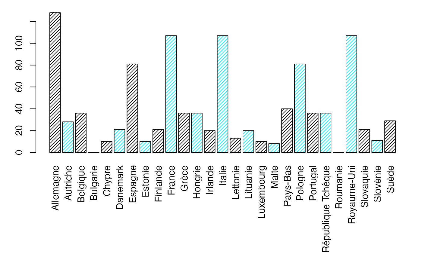
margX <- margin.table(Europ,1)
par(mar = c(3, 3, 1, 1) + 0.1, mgp = c(2, 1, 0))
mp <- barplot(margX, beside=FALSE, args.legend=list(x="topright"),col=c("black","cyan","black","cyan"),density=25) 
margY <- margin.table(Europ,2)
par(mar = c(9.1, 3, 1, 1) + 0.1, mgp = c(2, 1, 0))
mp <- barplot(margY, beside=FALSE, args.legend=list(x="topright"),col=c("black","cyan","black","cyan"),density=25,las=3) # default
Chemin <- "~/Documents/Recherche/DeBoeck/Graphes/Fichiers/"
colmodel="cmyk"
pdf(file = "SVeffmarg.pdf",
    width = 8, height = 7, onefile = TRUE, family = "Helvetica",
    title = "Probability or cumulative distribution graphs", paper = "special", colormodel = colmodel)
layout((1:2))
margX <- margin.table(Europ,1)
par(mar = c(3, 3, 1, 1) + 0.1, mgp = c(2, 1, 0))
mp <- barplot(margX, beside=FALSE, args.legend=list(x="topright"),col=c("black","cyan","black","cyan"),density=25) # default
margY <- margin.table(Europ,2)
par(mar = c(9.1, 3, 1, 1) + 0.1, mgp = c(2, 1, 0))
mp <- barplot(margY, beside=FALSE, args.legend=list(x="topright"),col=c("black","cyan","black","cyan"),density=25,las=3) # default
dev.off()
#> agg_png
#>       2
Chemin <- "~/Documents/Recherche/DeBoeck/Graphes/Fichiers/"
colmodel="cmyk"
pdf(file = "SVeffmargX.pdf",
    width = 8, height = 7, onefile = TRUE, family = "Helvetica",
    title = "Probability or cumulative distribution graphs", paper = "special", colormodel = colmodel)
margX <- margin.table(Europ,1)
par(mar = c(3, 3, 1, 1) + 0.1, mgp = c(2, 1, 0))
mp <- barplot(margX, beside=FALSE, args.legend=list(x="topright"),col=c("black","cyan","black","cyan"),density=25) # default
dev.off()
#> agg_png
#>       2
Chemin <- "~/Documents/Recherche/DeBoeck/Graphes/Fichiers/"
colmodel="cmyk"
pdf(file = "SVeffmargY.pdf",
    width = 8, height = 7, onefile = TRUE, family = "Helvetica",
    title = "Probability or cumulative distribution graphs", paper = "special", colormodel = colmodel)
margY <- margin.table(Europ,2)
par(mar = c(9.1, 3, 1, 1) + 0.1, mgp = c(2, 1, 0))
mp <- barplot(margY, beside=FALSE, args.legend=list(x="topright"),col=c("black","cyan","black","cyan"),density=25,las=3) # default
dev.off()
#> agg_png
#>       2
freqcondX <- prop.table(Europ,1) #Y|X
par(mar = c(3, 3, 1, 1) + 0.1, mgp = c(2, 1, 0))
mp <- barplot(t(freqcondX), beside=TRUE, legend = colnames(Europ), ylim = c(0, .35), args.legend=list(x="top", ncol=3)) # default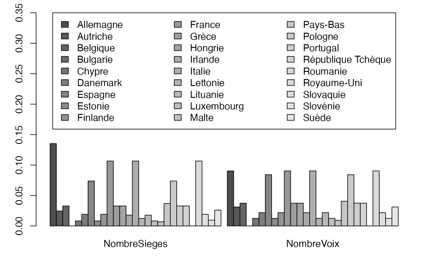
freqcondY <- prop.table(Europ,2) #Y|X
par(mar = c(9.1, 3, 1, 1) + 0.1, mgp = c(2, 1, 0))
mp <- barplot(freqcondY, beside=TRUE, legend = rownames(Europ), ylim = c(0, .95), args.legend=list(x="top", ncol=2),las=3) # default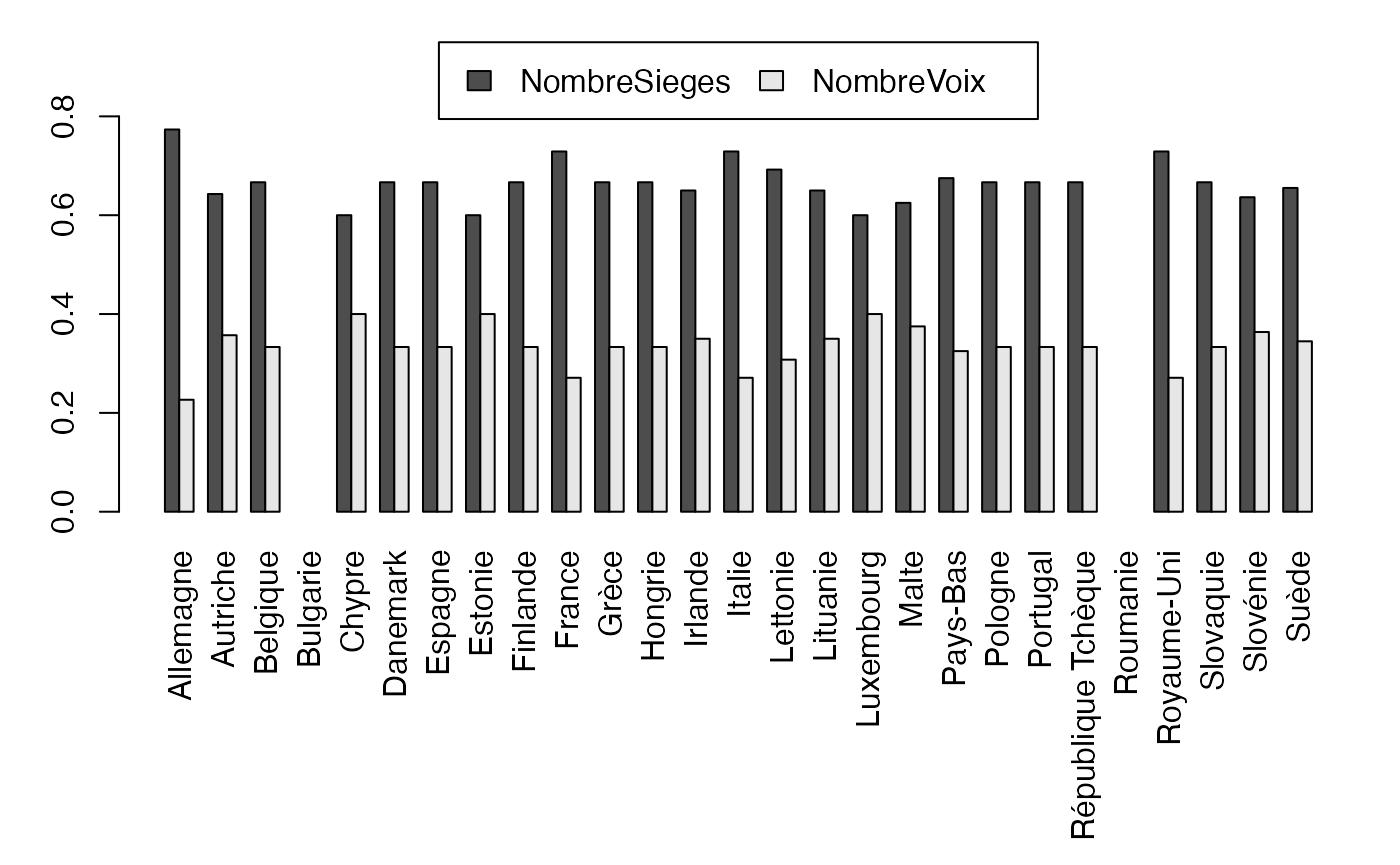
Chemin <- "~/Documents/Recherche/DeBoeck/Graphes/Fichiers/"
colmodel="cmyk"
pdf(file = "SVfrecondBesideX.pdf",
    width = 8, height = 7, onefile = TRUE, family = "Helvetica",
    title = "Probability or cumulative distribution graphs", paper = "special", colormodel = colmodel)
freqcondX <- prop.table(Europ,1) #Y|X
par(mar = c(3, 3, 1, 1) + 0.1, mgp = c(2, 1, 0))
mp <- barplot(t(freqcondX), beside=TRUE, legend = colnames(Europ), ylim = c(0, .22), args.legend=list(x="top", ncol=3)) # default
dev.off()
#> agg_png
#>       2
Chemin <- "~/Documents/Recherche/DeBoeck/Graphes/Fichiers/"
colmodel="cmyk"
pdf(file = "SVfrecondBesideY.pdf",
    width = 8, height = 7, onefile = TRUE, family = "Helvetica",
    title = "Probability or cumulative distribution graphs", paper = "special", colormodel = colmodel)
freqcondY <- prop.table(Europ,2) #Y|X
par(mar = c(9.1, 3, 1, 1) + 0.1, mgp = c(2, 1, 0))
mp <- barplot(freqcondY, beside=TRUE, legend = rownames(Europ), ylim = c(0, .85), args.legend=list(x="top", ncol=2),las=3) # default
dev.off()
#> agg_png
#>       2
freqcondX <- prop.table(Europ,1) #Y|X
par(mar = c(3, 3, 1, 1) + 0.1, mgp = c(2, 1, 0))
mp <- barplot(t(freqcondX), beside=FALSE, legend = colnames(Europ), ylim = c(0, 1.6), args.legend=list(x="top", ncol=3),yaxt="n") # default
axis(2, at=0:5*.2)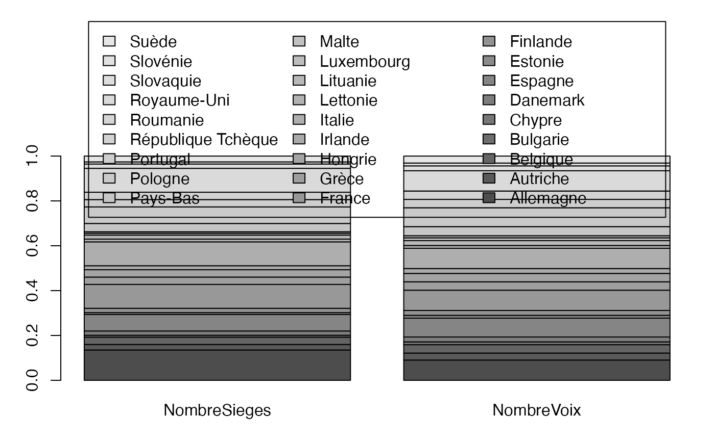
freqcondY <- prop.table(Europ,2) #Y|X
par(mar = c(9.1, 3, 1, 1) + 0.1, mgp = c(2, 1, 0))
mp <- barplot(freqcondY, beside=FALSE, legend = rownames(Europ), ylim = c(0, 1.3), args.legend=list(x="top", ncol=4),yaxt="n",las=3) # default
axis(2, at=0:5*.2)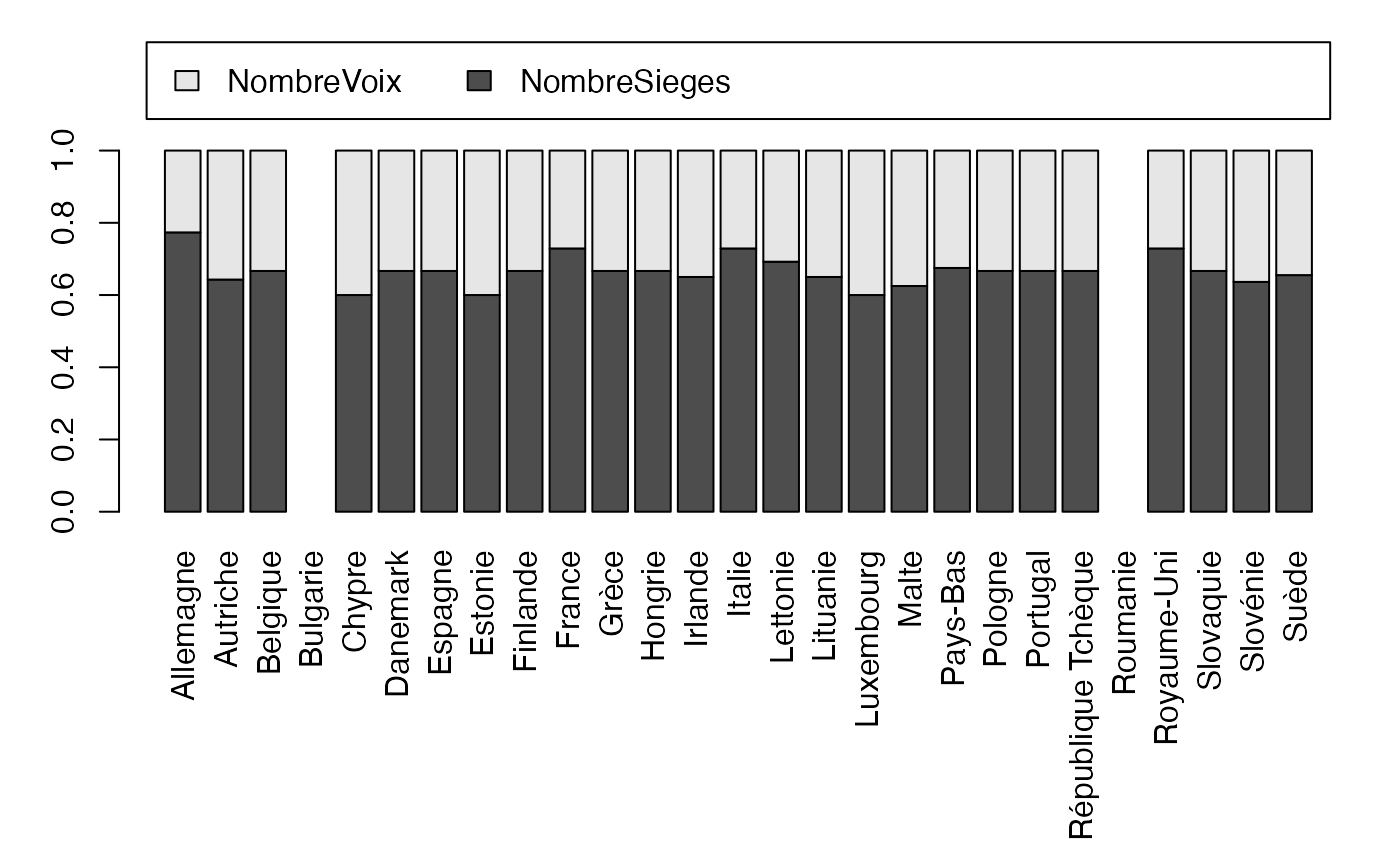
Chemin <- "~/Documents/Recherche/DeBoeck/Graphes/Fichiers/"
colmodel="cmyk"
pdf(file = "SVfrecondStackedX.pdf",
    width = 8, height = 7, onefile = TRUE, family = "Helvetica",
    title = "Probability or cumulative distribution graphs", paper = "special", colormodel = colmodel)
freqcondX <- prop.table(Europ,1) #Y|X
par(mar = c(3, 3, 1, 1) + 0.1, mgp = c(2, 1, 0))
mp <- barplot(t(freqcondX), beside=FALSE, legend = colnames(Europ), ylim = c(0, 1.6), args.legend=list(x="top", ncol=3),yaxt="n") # default
axis(2, at=0:5*.2)
dev.off()
#> agg_png
#>       2
Chemin <- "~/Documents/Recherche/DeBoeck/Graphes/Fichiers/"
colmodel="cmyk"
pdf(file = "SVfrecondStackedY.pdf",
    width = 8, height = 7, onefile = TRUE, family = "Helvetica",
    title = "Probability or cumulative distribution graphs", paper = "special", colormodel = colmodel)
freqcondY <- prop.table(Europ,2) #Y|X
par(mar = c(9.1, 3, 1, 1) + 0.1, mgp = c(2, 1, 0))
mp <- barplot(freqcondY, beside=FALSE, legend = rownames(Europ), ylim = c(0, 1.3), args.legend=list(x="top", ncol=4),yaxt="n",las=3) # default
axis(2, at=0:5*.2)
dev.off()
#> agg_png
#>       2
Muldimensionnel
ggpairs
if(!("GGally" %in% installed.packages())){install.packages("GGally")}
library(GGally)
#> Loading required package: ggplot2
ggpairs(iris, progress = FALSE)
#> `stat_bin()` using `bins = 30`. Pick better value `binwidth`.
#> `stat_bin()` using `bins = 30`. Pick better value `binwidth`.
#> `stat_bin()` using `bins = 30`. Pick better value `binwidth`.
#> `stat_bin()` using `bins = 30`. Pick better value `binwidth`.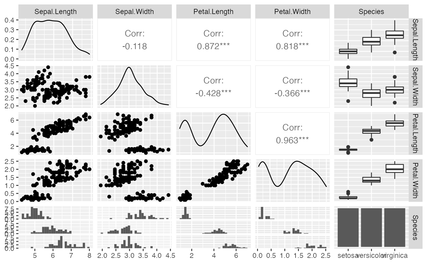
Chemin <- "~/Documents/Recherche/DeBoeck/Graphes/Fichiers/"
colmodel="cmyk"
ggsave(filename = paste(Chemin,"Iris_ggpairs.pdf",sep=""),
       width = 16, height = 10, onefile = TRUE, family = "Helvetica", title = "Probability or cumulative distribution graphs", paper = "special", colormodel = colmodel)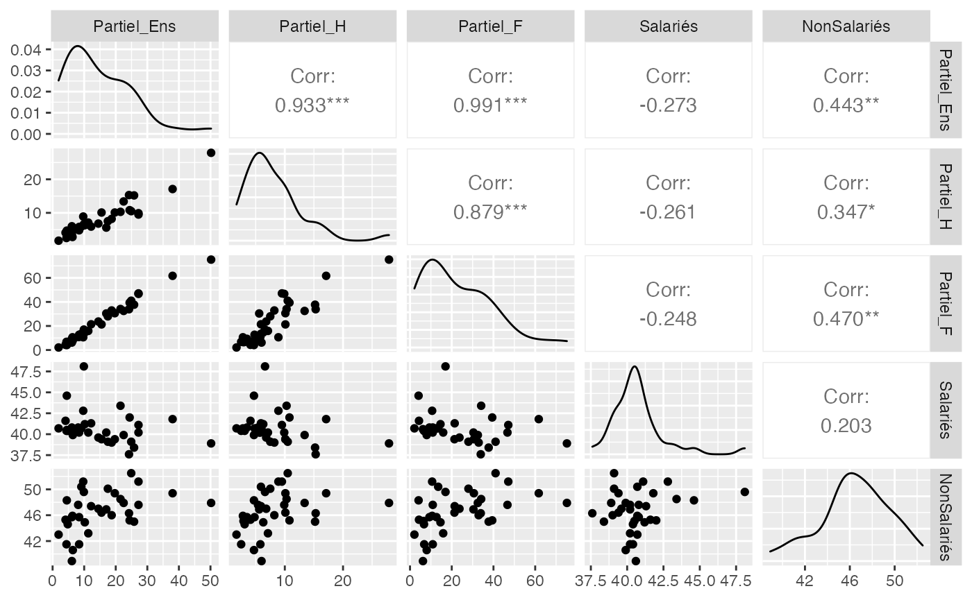
Chemin <- "~/Documents/Recherche/DeBoeck/Graphes/Fichiers/"
colmodel="cmyk"
ggsave(filename = paste(Chemin,"Europe_ggpairs.pdf",sep=""),
       width = 16, height = 10, onefile = TRUE, family = "Helvetica",
    title = "Probability or cumulative distribution graphs", paper = "special", colormodel = colmodel)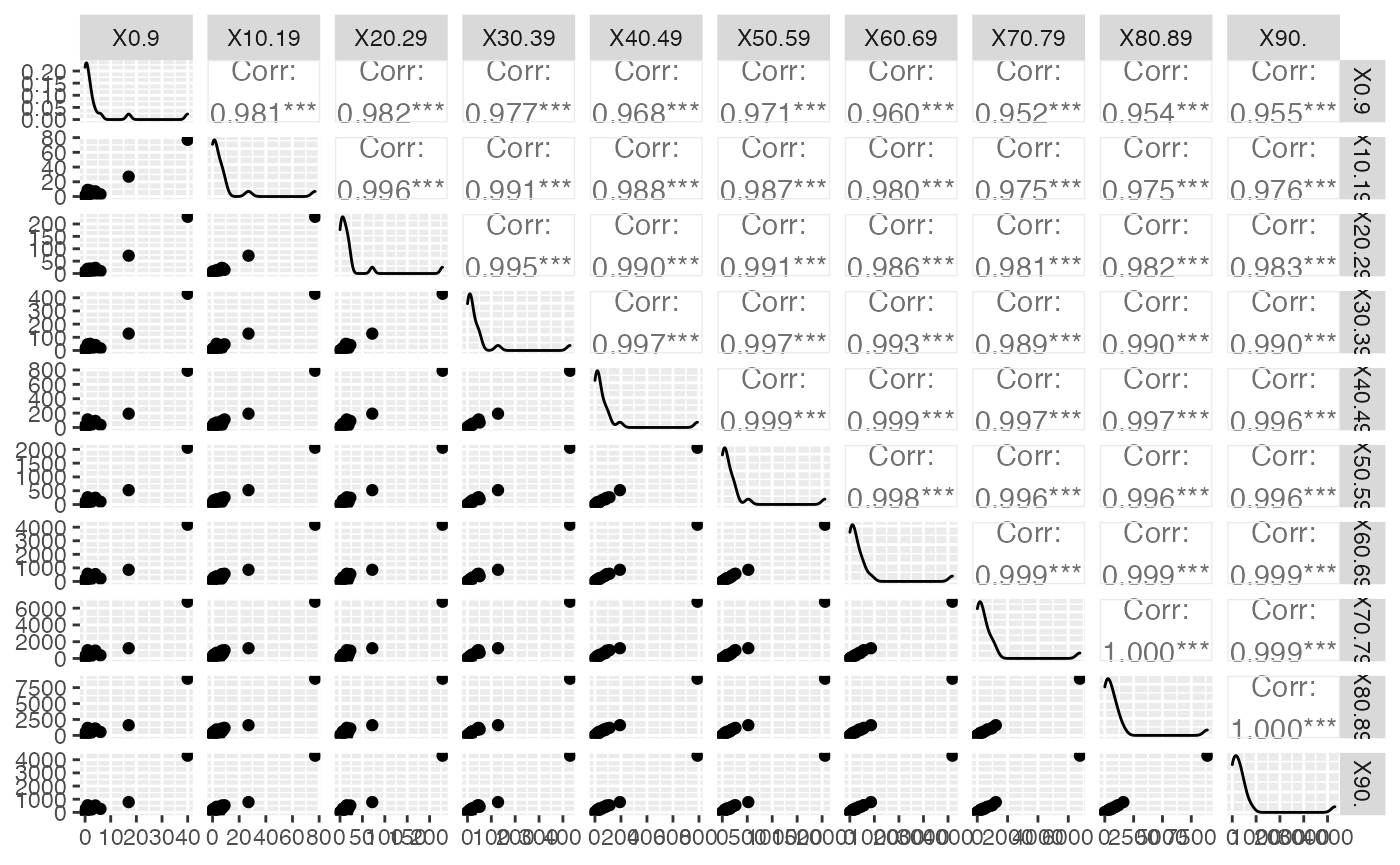
Chemin <- "~/Documents/Recherche/DeBoeck/Graphes/Fichiers/"
colmodel="cmyk"
ggsave(filename = paste(Chemin,"Hospit_ggpairs.pdf",sep=""),
       width = 16, height = 10, onefile = TRUE, family = "Helvetica",
    title = "Probability or cumulative distribution graphs", paper = "special", colormodel = colmodel)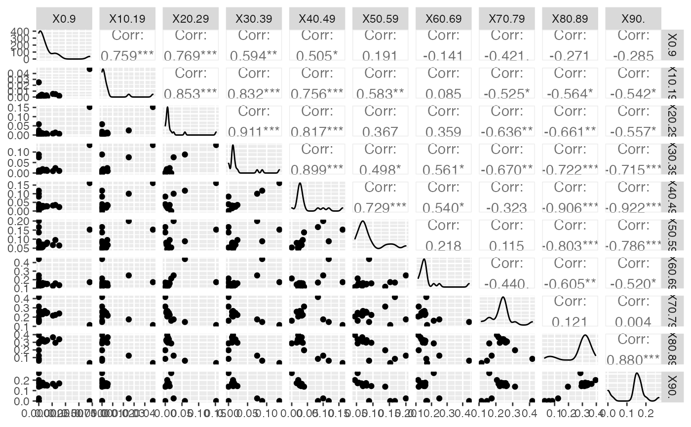
Chemin <- "~/Documents/Recherche/DeBoeck/Graphes/Fichiers/"
colmodel="cmyk"
ggsave(filename = paste(Chemin,"Hospit_Norm_ggpairs.pdf",sep=""),
       width = 16, height = 10, onefile = TRUE, family = "Helvetica",
    title = "Probability or cumulative distribution graphs", paper = "special", colormodel = colmodel)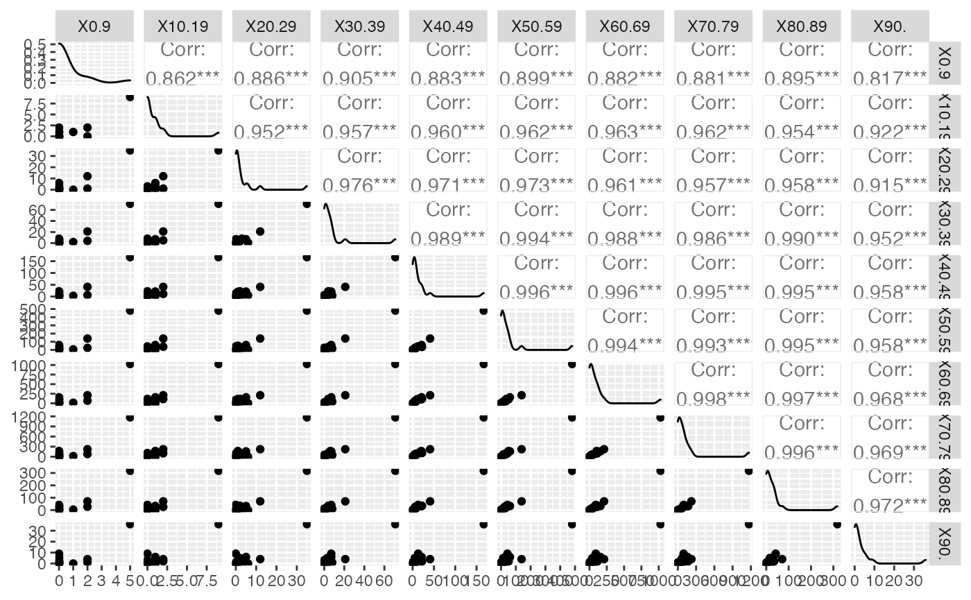
Chemin <- "~/Documents/Recherche/DeBoeck/Graphes/Fichiers/"
colmodel="cmyk"
ggsave(filename = paste(Chemin,"Rea_ggpairs.pdf",sep=""),
       width = 16, height = 10, onefile = TRUE, family = "Helvetica",
    title = "Probability or cumulative distribution graphs", paper = "special", colormodel = colmodel)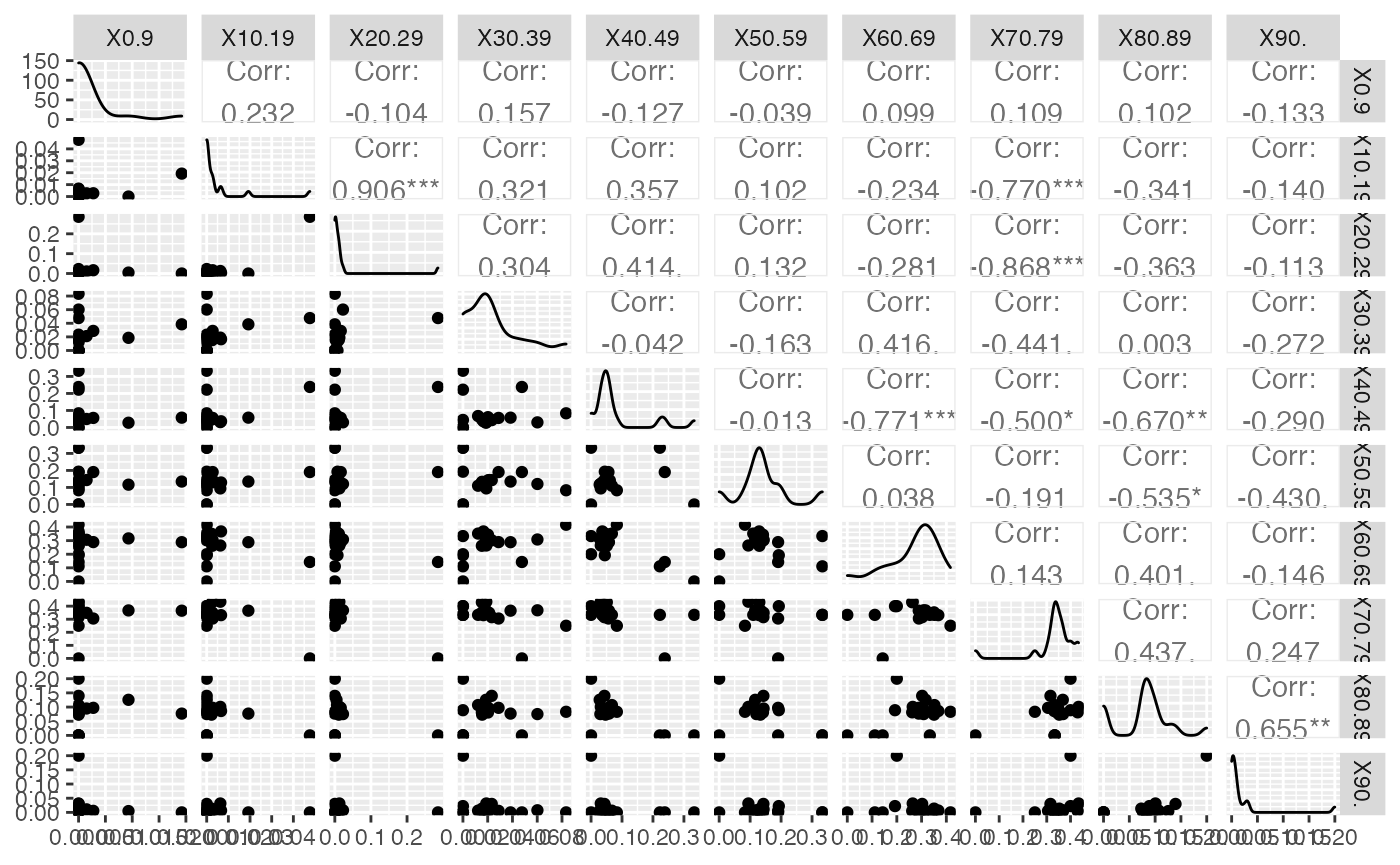
Chemin <- "~/Documents/Recherche/DeBoeck/Graphes/Fichiers/"
colmodel="cmyk"
ggsave(filename = paste(Chemin,"Rea_Norm_ggpairs.pdf",sep=""),
       width = 16, height = 10, onefile = TRUE, family = "Helvetica",
    title = "Probability or cumulative distribution graphs", paper = "special", colormodel = colmodel)
Radar Plots
if(!("ggplot2" %in% installed.packages())){install.packages("ggplot2")}
library(ggplot2)
if(!("ggiraphExtra" %in% installed.packages())){install.packages("ggiraphExtra")}
library(ggiraphExtra)
ggiraphExtra::ggRose(rose,ggplot2::aes(x=Month,fill=group,y=value),stat="identity",interactive=TRUE)
#> Warning: `aes_string()` was deprecated in ggplot2 3.0.0.
#> ℹ Please use tidy evaluation idioms with `aes()`.
#> ℹ See also `vignette("ggplot2-in-packages")` for more information.
#> ℹ The deprecated feature was likely used in the ggiraphExtra package.
#>   Please report the issue to the authors.
#> This warning is displayed once every 8 hours.
#> Call `lifecycle::last_lifecycle_warnings()` to see where this warning was
#> generated.
#> Warning in (function (mapping = NULL, data = NULL, stat = "count", position =
#> "stack", : Ignoring unknown parameters: `size`
if(!("moonBook" %in% installed.packages())){install.packages("moonBook")}
library(moonBook)
#>
#> Attaching package: 'moonBook'
#> The following objects are masked from 'package:ggiraphExtra':
#>
#>     addLabelDf, getMapping
#> The following object is masked from 'package:lattice':
#>
#>     densityplot
ggiraphExtra::ggRose(acs,ggplot2::aes(x=Dx,fill=smoking),interactive=TRUE)
#> Warning in (function (mapping = NULL, data = NULL, stat = "count", position =
#> "stack", : Ignoring unknown parameters: `size`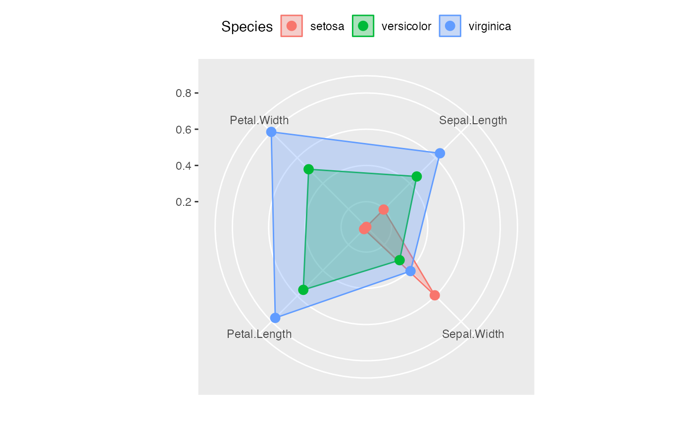
if(!("ggplot2" %in% installed.packages())){install.packages("ggplot2")}
library(ggplot2)
if(!("ggradar" %in% installed.packages())){
devtools::install_github("ricardo-bion/ggradar", dependencies=TRUE)
}
library(ggradar)
#>
#> Attaching package: 'ggradar'
#> The following object is masked from 'package:sageR':
#>
#>     ggradar
if(!("dplyr" %in% installed.packages())){install.packages("dplyr")}
suppressPackageStartupMessages(library(dplyr))
if(!("scales" %in% installed.packages())){install.packages("scales")}
library(scales)
#>
#> Attaching package: 'scales'
#> The following object is masked from 'package:moonBook':
#>
#>     comma
ggradar(data.frame(levels(iris[,5]),t(simplify2array(lapply(split(iris[,-5],iris[,5]),colMeans))/apply(simplify2array(lapply(split(iris[,-5],iris[,5]),colMeans)),1,max))),axis.labels = c("Sepal Length","Sepal\nWidth","Petal Length","Petal\nWidth"))
#> Ignoring unknown labels:
#> • size : "14"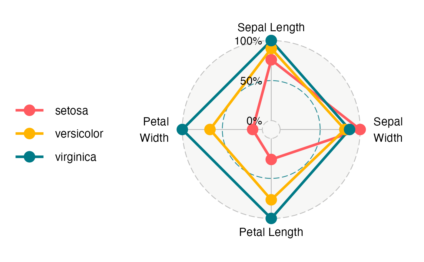
Chemin <- "~/Documents/Recherche/DeBoeck/Graphes/Fichiers/"
colmodel="cmyk"
ggsave(filename = paste(Chemin,"Iris_ggradar.pdf",sep=""),
       width = 8, height = 7, onefile = TRUE, family = "Helvetica", title = "Probability or cumulative distribution graphs", paper = "special", colormodel = colmodel)
data(Europe)

Europe_rad <- Europe[,-1]
rownames(Europe_rad) <- Europe[,1]

Europe_radar <- Europe_rad %>%
  as_tibble(rownames = "group") %>%
  mutate_at(vars(-group), rescale)
Europe_radar
#> # A tibble: 35 × 6
#>    group     Partiel_Ens Partiel_H Partiel_F Salariés NonSalariés
#>    <chr>           <dbl>     <dbl>     <dbl>    <dbl>       <dbl>
#>  1 Allemagne      0.524     0.313     0.610     0.248       0.640
#>  2 Autriche       0.524     0.298     0.616     0.333       0.904
#>  3 Belgique       0.476     0.336     0.532     0.143       1
#>  4 Bulgarie       0         0         0         0.295       0.301
#>  5 Chypre         0.172     0.176     0.171     0.343       0.441
#>  6 Croatie        0.0600    0.0534    0.0629    0.267       0.419
#>  7 Danemark       0.462     0.519     0.435     0           0.544
#>  8 Espagne        0.261     0.195     0.295     0.190       0.596
#>  9 Estonie        0.195     0.206     0.189     0.248       0.316
#> 10 Finlande       0.282     0.321     0.263     0.171       0.551
#> # ℹ 25 more rows
ggradar(Europe_radar,axis.labels = c("Partiel Ens.", "Partiel\nHommes",   "Partiel\nFemmes",   "Salariés","Non\nSalariés"), legend.text.size=10)
#> Ignoring unknown labels:
#> • size : "10"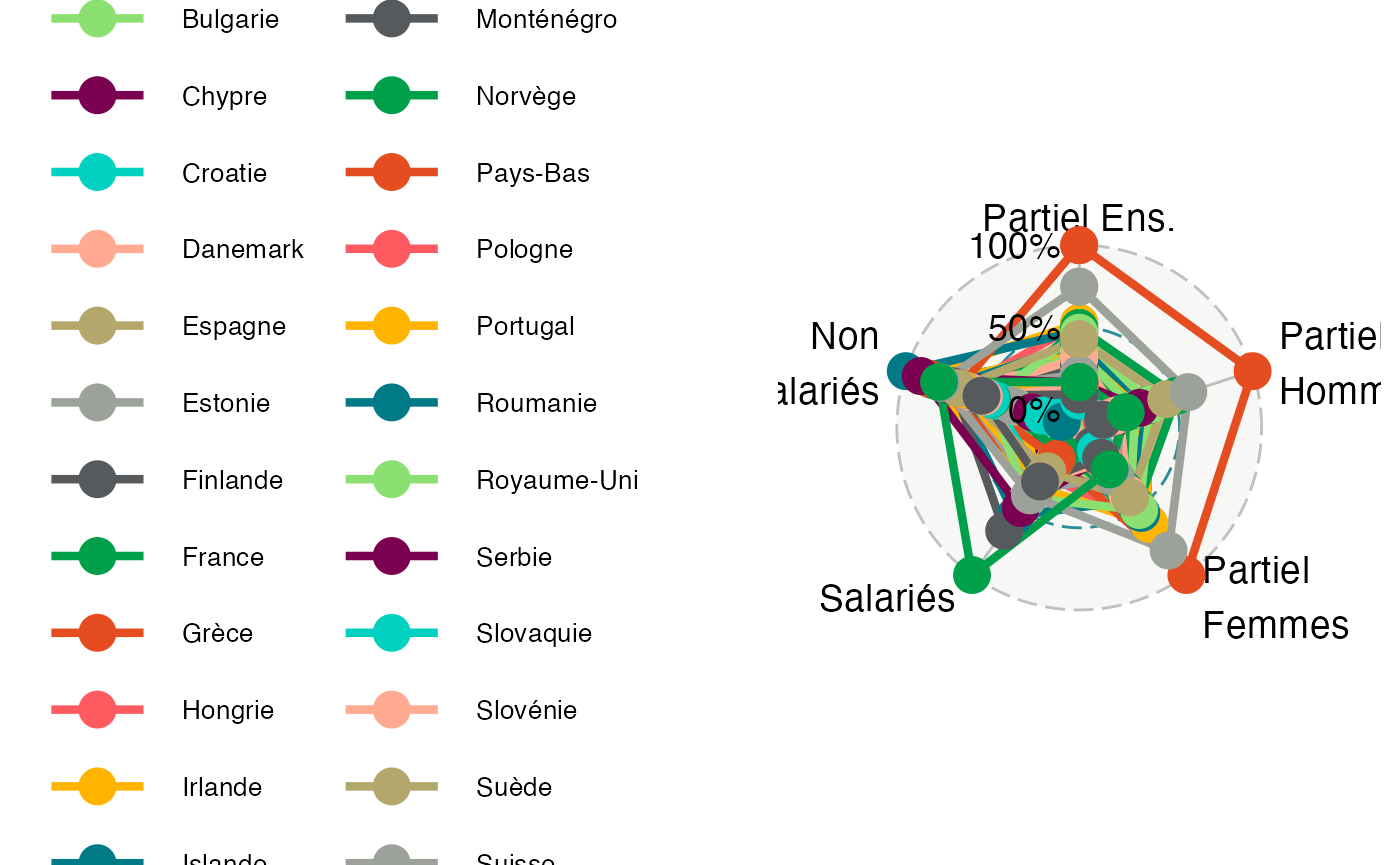
Chemin <- "~/Documents/Recherche/DeBoeck/Graphes/Fichiers/"
colmodel="cmyk"
ggsave(filename = paste(Chemin,"Europe_ggradar.pdf",sep=""),
       width = 16, height = 10, onefile = TRUE, family = "Helvetica",
    title = "Probability or cumulative distribution graphs", paper = "special", colormodel = colmodel)
data(HospitFull)
Hospit=cbind(Région=(HospitFull$Région)[-nrow(HospitFull)],HospitFull[-nrow(ReaFull),-c(1,2)])
summary(Hospit)
#>     Région               X0.9            X10.19           X20.29
#>  Length:18          Min.   : 0.000   Min.   : 0.000   Min.   : 0.00
#>  Class :character   1st Qu.: 0.000   1st Qu.: 0.000   1st Qu.: 3.00
#>  Mode  :character   Median : 1.000   Median : 2.500   Median : 9.00
#>                     Mean   : 2.222   Mean   : 4.278   Mean   :12.72
#>                     3rd Qu.: 2.000   3rd Qu.: 6.500   3rd Qu.:15.75
#>                     Max.   :17.000   Max.   :27.000   Max.   :72.00
#>      X30.39           X40.49           X50.59          X60.69
#>  Min.   :  0.00   Min.   :  0.00   Min.   :  2.0   Min.   :  2.00
#>  1st Qu.:  4.00   1st Qu.:  7.25   1st Qu.: 10.0   1st Qu.: 15.75
#>  Median : 15.00   Median : 28.00   Median : 81.0   Median :184.50
#>  Mean   : 23.89   Mean   : 43.83   Mean   :114.3   Mean   :232.28
#>  3rd Qu.: 34.25   3rd Qu.: 64.75   3rd Qu.:179.5   3rd Qu.:359.75
#>  Max.   :128.00   Max.   :192.00   Max.   :521.0   Max.   :861.00
#>      X70.79           X80.89            X90.
#>  Min.   :   5.0   Min.   :   1.0   Min.   :  0.0
#>  1st Qu.:  13.0   1st Qu.:  11.5   1st Qu.:  9.0
#>  Median : 296.0   Median : 418.0   Median :221.0
#>  Mean   : 376.1   Mean   : 494.3   Mean   :239.3
#>  3rd Qu.: 599.8   3rd Qu.: 798.0   3rd Qu.:382.5
#>  Max.   :1222.0   Max.   :1607.0   Max.   :783.0

Hospit_rad <- Hospit[,-1]
rownames(Hospit_rad) <- Hospit[,1]

Hospit_radar <- Hospit_rad %>%
  as_tibble(rownames = "group") %>%
  mutate_at(vars(-group), rescale)
Hospit_radar
#> # A tibble: 18 × 11
#>    group       X0.9 X10.19 X20.29 X30.39  X40.49  X50.59  X60.69  X70.79  X80.89
#>    <chr>      <dbl>  <dbl>  <dbl>  <dbl>   <dbl>   <dbl>   <dbl>   <dbl>   <dbl>
#>  1 Ile-de-F… 1      1      1      1      1       1       1       1       1   e+0
#>  2 Auvergne… 0.0588 0.333  0.208  0.367  0.583   0.503   0.662   0.809   7.39e-1
#>  3 Provence… 0.235  0.259  0.319  0.328  0.474   0.470   0.633   0.767   6.77e-1
#>  4 Grand-Est 0.118  0.111  0.181  0.398  0.359   0.366   0.445   0.554   5.84e-1
#>  5 Hauts-de… 0.118  0.296  0.278  0.305  0.422   0.358   0.501   0.523   5.32e-1
#>  6 Occitanie 0.176  0.0370 0.0833 0.156  0.271   0.293   0.332   0.385   3.88e-1
#>  7 Bourgogn… 0.0588 0.259  0.264  0.148  0.177   0.177   0.274   0.351   3.70e-1
#>  8 Nouvelle… 0.353  0.111  0.139  0.125  0.188   0.193   0.247   0.304   3.31e-1
#>  9 Normandie 0.0588 0.0741 0.153  0.148  0.167   0.145   0.251   0.255   2.71e-1
#> 10 Centre-V… 0      0      0.111  0.0781 0.0885  0.160   0.178   0.224   1.97e-1
#> 11 Pays de … 0      0      0.0833 0.0938 0.109   0.0848  0.133   0.168   2.48e-1
#> 12 Bretagne  0.118  0.148  0.0833 0.0547 0.125   0.0944  0.111   0.130   1.71e-1
#> 13 Mayotte   0.0588 0.185  0.222  0.109  0.0885  0.0270  0.0186  0.00575 1.25e-3
#> 14 Corse     0      0      0.0139 0      0       0.00193 0.0116  0.00329 9.34e-3
#> 15 Guadelou… 0      0      0      0      0.0104  0.00963 0.00466 0.00904 5.60e-3
#> 16 La Réuni… 0      0.0370 0.0139 0.0234 0.0208  0.0116  0.00931 0.00164 2.49e-3
#> 17 Guyane    0      0      0.0278 0.0234 0.0208  0.00193 0.0151  0       6.23e-4
#> 18 Martiniq… 0      0      0      0      0.00521 0       0       0       0
#> # ℹ 1 more variable: X90. <dbl>
ggradar(Hospit_radar, legend.text.size=12)
#> Ignoring unknown labels:
#> • size : "12"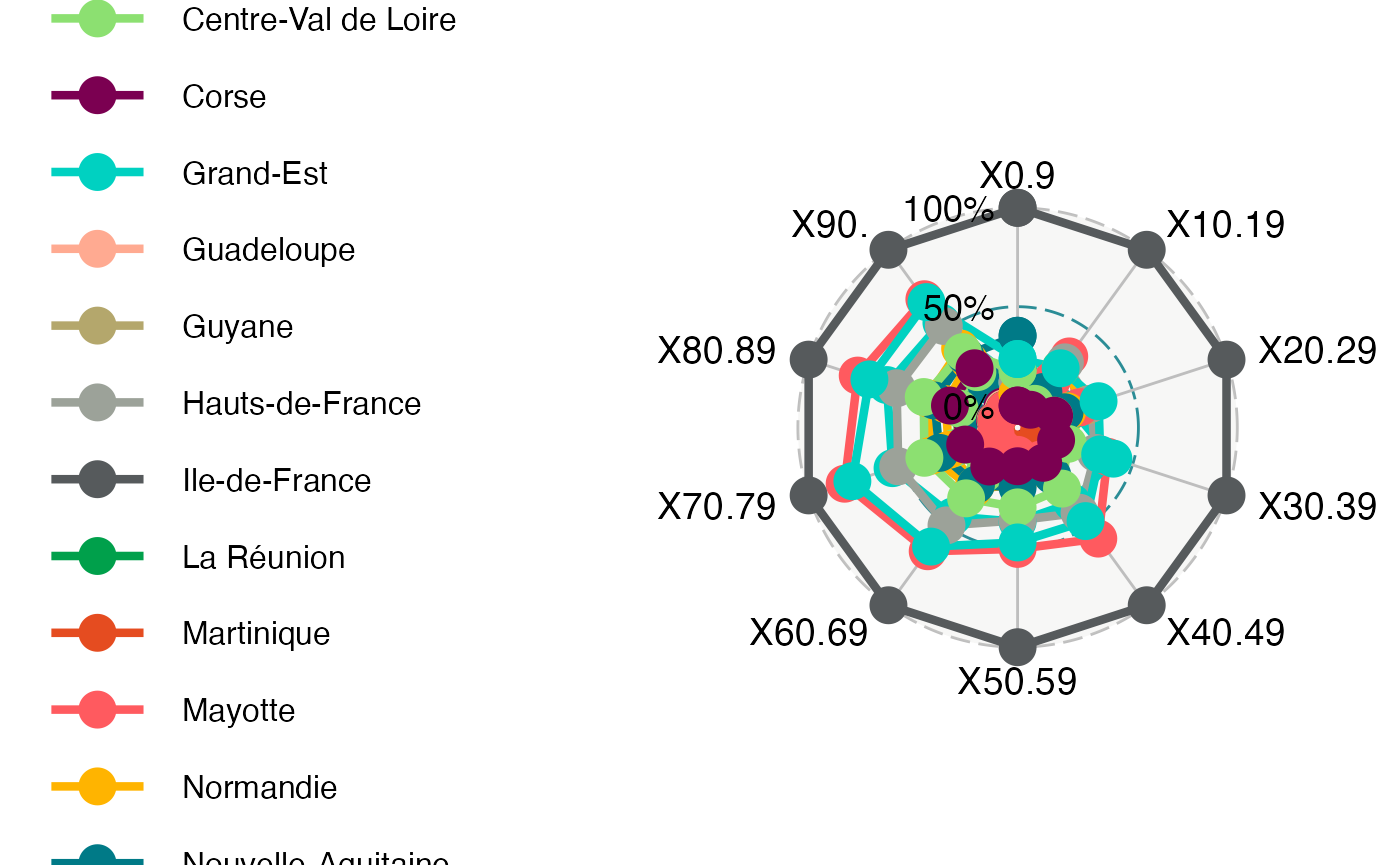
Chemin <- "~/Documents/Recherche/DeBoeck/Graphes/Fichiers/"
colmodel="cmyk"
ggsave(filename = paste(Chemin,"Hospit_ggradar.pdf",sep=""),
       width = 16, height = 10, onefile = TRUE, family = "Helvetica",
    title = "Probability or cumulative distribution graphs", paper = "special", colormodel = colmodel)
data(ReaFull)
Rea=cbind(Région=(ReaFull$Région)[-nrow(ReaFull)],ReaFull[-nrow(ReaFull),-c(1,2)])
summary(Rea)
#>     Région               X0.9            X10.19        X20.29
#>  Length:18          Min.   :0.0000   Min.   :0.0   Min.   : 0.000
#>  Class :character   1st Qu.:0.0000   1st Qu.:0.0   1st Qu.: 0.000
#>  Mode  :character   Median :0.0000   Median :0.0   Median : 1.000
#>                     Mean   :0.2778   Mean   :0.5   Mean   : 1.944
#>                     3rd Qu.:0.0000   3rd Qu.:1.0   3rd Qu.: 2.000
#>                     Max.   :2.0000   Max.   :2.0   Max.   :12.000
#>      X30.39           X40.49           X50.59           X60.69
#>  Min.   : 0.000   Min.   : 0.000   Min.   :  0.00   Min.   :  0.00
#>  1st Qu.: 0.250   1st Qu.: 2.250   1st Qu.:  3.25   1st Qu.:  3.50
#>  Median : 2.500   Median : 5.500   Median : 15.50   Median : 37.50
#>  Mean   : 3.944   Mean   : 9.278   Mean   : 26.72   Mean   : 57.06
#>  3rd Qu.: 5.750   3rd Qu.:12.500   3rd Qu.: 38.25   3rd Qu.:100.00
#>  Max.   :21.000   Max.   :41.000   Max.   :139.00   Max.   :211.00
#>      X70.79           X80.89           X90.
#>  Min.   :  0.00   Min.   : 0.00   Min.   :0.00
#>  1st Qu.:  3.00   1st Qu.: 1.00   1st Qu.:0.00
#>  Median : 51.50   Median :11.00   Median :1.00
#>  Mean   : 65.00   Mean   :17.67   Mean   :2.00
#>  3rd Qu.: 98.75   3rd Qu.:30.75   3rd Qu.:2.75
#>  Max.   :223.00   Max.   :71.00   Max.   :9.00

Rea_rad <- Rea[,-1]
rownames(Rea_rad) <- Rea[,1]

Rea_radar <- Rea_rad %>%
  as_tibble(rownames = "group") %>%
  mutate_at(vars(-group), rescale)
Rea_radar
#> # A tibble: 18 × 11
#>    group   X0.9 X10.19 X20.29 X30.39 X40.49  X50.59  X60.69  X70.79 X80.89  X90.
#>    <chr>  <dbl>  <dbl>  <dbl>  <dbl>  <dbl>   <dbl>   <dbl>   <dbl>  <dbl> <dbl>
#>  1 Ile-d…   1      1   1      1      1      1       1       1       1      0.444
#>  2 Prove…   0      0.5 0.417  0.333  0.512  0.432   0.749   0.713   0.465  0.667
#>  3 Auver…   0      0.5 0.0833 0.286  0.488  0.367   0.488   0.758   0.451  0.222
#>  4 Grand…   0      0   0.167  0.190  0.537  0.259   0.545   0.489   0.493  0.222
#>  5 Hauts…   0      1   0.0833 0.238  0.268  0.281   0.526   0.448   0.366  0.222
#>  6 Occit…   0      0   0      0.333  0.317  0.309   0.431   0.426   0.592  1
#>  7 Nouve…   1      0   0.0833 0.190  0.146  0.180   0.322   0.354   0.380  0.111
#>  8 Bourg…   0      0.5 0.167  0.143  0.122  0.108   0.199   0.309   0.225  0.556
#>  9 Centr…   0      0   0.0833 0      0.146  0.187   0.123   0.242   0.169  0.333
#> 10 Norma…   0      0   0.25   0.381  0.0976 0.115   0.194   0.220   0.141  0.111
#> 11 Pays …   0      0   0.0833 0.0952 0.146  0.101   0.161   0.152   0.113  0
#> 12 Breta…   0.5    0.5 0      0.0952 0.0732 0.0504  0.0711  0.0852  0.0563 0
#> 13 Mayot…   0      0.5 0.5    0.0476 0.122  0.0288  0.0142  0       0      0
#> 14 Guyane   0      0   0      0.0476 0.0244 0.00719 0.0237  0.0135  0.0141 0
#> 15 La Ré…   0      0   0      0      0.0488 0.0216  0.00474 0.0135  0      0
#> 16 Guade…   0      0   0      0      0      0.0144  0.00948 0.00897 0      0
#> 17 Corse    0      0   0      0      0      0       0.00474 0.00897 0.0141 0.111
#> 18 Marti…   0      0   0      0      0.0244 0       0       0.00448 0      0
ggradar(Rea_radar, legend.text.size=12)
#> Ignoring unknown labels:
#> • size : "12"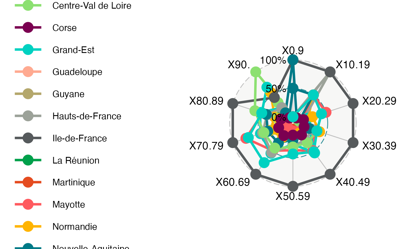
Chernov Faces
if(!("DescTools" %in% installed.packages())){install.packages("DescTools")}
library(DescTools)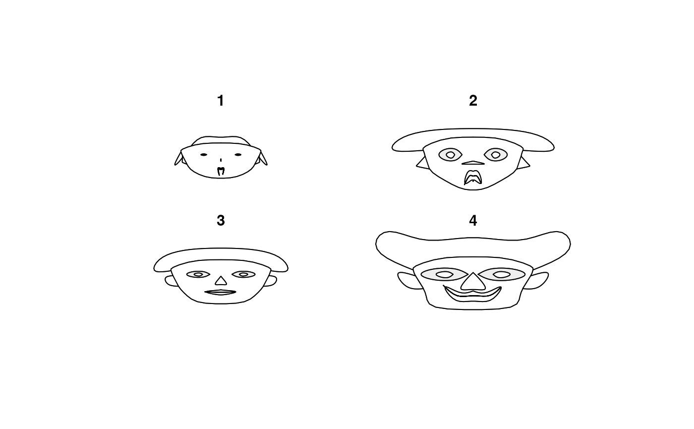
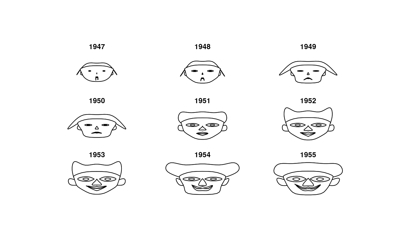

means <- lapply(iris[,-5], tapply, iris$Species, mean)
m <- t(do.call(rbind, means))
m <- cbind(m, matrix(rep(1, 11*3), nrow=3))

# define the colors, first for all faces the same
col <- replicate(3, c("orchid1", "olivedrab", "goldenrod4",
                      "peachpuff", "darksalmon", "peachpuff3"))
rownames(col) <- c("nose","eyes","hair","face","lips","ears")
# change haircolor individually for each face
col[3, ] <- c("lightgoldenrod", "coral3", "sienna4")

z <- PlotFaces(m, nr=1, nc=3, col=col)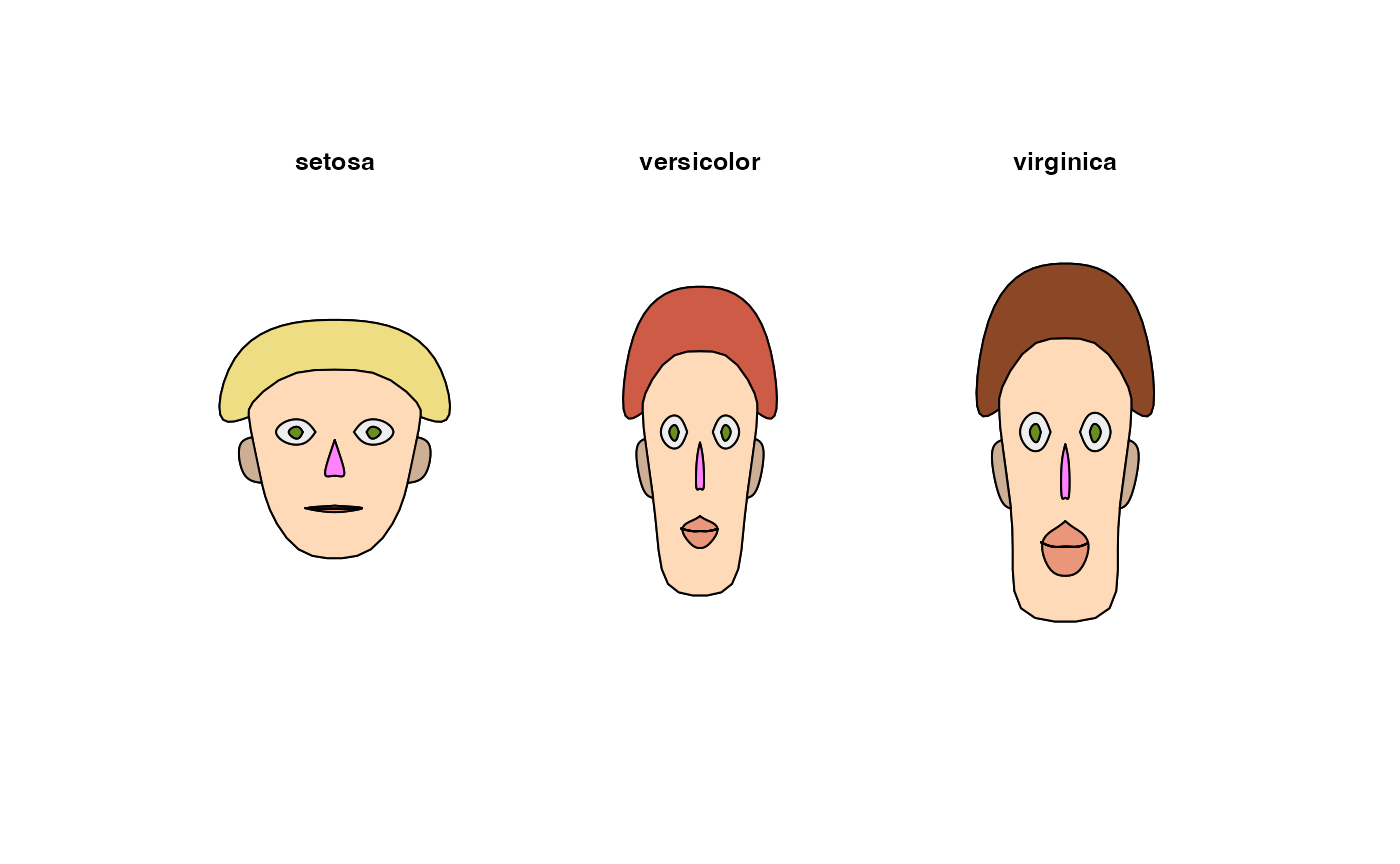
# print the used coding
print(z$info, right=FALSE)
#>    modified.item     variable
#> 1  height of face    Sepal.Length
#> 2  width of face     Sepal.Width
#> 3  structure of face Petal.Length
#> 4  height of mouth   Petal.Width
#> 5  width of mouth
#> 6  smiling
#> 7  height of eyes
#> 8  width of eyes
#> 9  height of hair
#> 10 width of hair
#> 11 style of hair
#> 12 height of nose
#> 13 width of nose
#> 14 width of ear
#> 15 height of ear
Chemin <- "~/Documents/Recherche/DeBoeck/Graphes/Fichiers/"
colmodel="cmyk"
pdf(file = "IrisChernoff.pdf",
    width = 8, height = 7, onefile = TRUE, family = "Helvetica",
    title = "Probability or cumulative distribution graphs", paper = "special", colormodel = colmodel)
par(mar = c(3, 3, 1, 1) + 0.1, mgp = c(2, 1, 0))
PlotFaces(m, nr=1, nc=3, col=col)
dev.off()
#> agg_png
#>       2
data(Europe)

means <- lapply(Europe[,-1], tapply, Europe$Etats.membres, mean)
m1 <- t(do.call(rbind, means))
# Complétion car au plus 15 variables
m <- cbind(m1, matrix(rep(1, (15-ncol(m1))*nrow(m1)), nrow=nrow(m1)))

# define the colors, first for all faces the same
col <- replicate(nrow(m1), c("orchid1", "olivedrab", "goldenrod4", "peachpuff", "darksalmon", "peachpuff3"))
rownames(col) <- c("nose","eyes","hair","face","lips","ears")
# change haircolor individually for each face
# col[3, ] <- c("lightgoldenrod", "coral3", "sienna4")
set.seed(4669)
col[3, ] <- sample(colors(),nrow(m1))
z <- PlotFaces(m, nr=6, nc=6, col=col)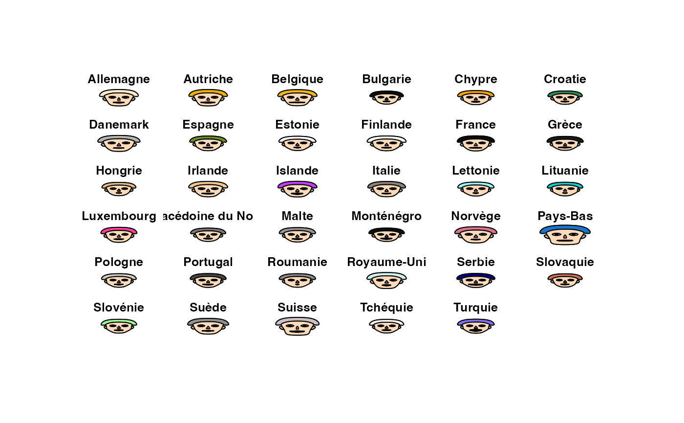
# print the used coding
print(z$info, right=FALSE)
#>    modified.item     variable
#> 1  height of face    Partiel_Ens
#> 2  width of face     Partiel_H
#> 3  structure of face Partiel_F
#> 4  height of mouth   Salariés
#> 5  width of mouth    NonSalariés
#> 6  smiling
#> 7  height of eyes
#> 8  width of eyes
#> 9  height of hair
#> 10 width of hair
#> 11 style of hair
#> 12 height of nose
#> 13 width of nose
#> 14 width of ear
#> 15 height of ear
Chemin <- "~/Documents/Recherche/DeBoeck/Graphes/Fichiers/"
colmodel="cmyk"
pdf(file = "EuropeChernoff.pdf",
    width = 14, height = 10, onefile = TRUE, family = "Helvetica",
    title = "Probability or cumulative distribution graphs", paper = "special", colormodel = colmodel)
par(mar = c(3, 3, 1, 1) + 0.1, mgp = c(2, 1, 0))
PlotFaces(m, nr=6, nc=6, col=col)
dev.off()
#> agg_png
#>       2
data(ReaFull)
Rea=cbind(Région=(ReaFull$Région)[-nrow(ReaFull)],ReaFull[-nrow(ReaFull),-c(1,2)])
summary(Rea)
#>     Région               X0.9            X10.19        X20.29
#>  Length:18          Min.   :0.0000   Min.   :0.0   Min.   : 0.000
#>  Class :character   1st Qu.:0.0000   1st Qu.:0.0   1st Qu.: 0.000
#>  Mode  :character   Median :0.0000   Median :0.0   Median : 1.000
#>                     Mean   :0.2778   Mean   :0.5   Mean   : 1.944
#>                     3rd Qu.:0.0000   3rd Qu.:1.0   3rd Qu.: 2.000
#>                     Max.   :2.0000   Max.   :2.0   Max.   :12.000
#>      X30.39           X40.49           X50.59           X60.69
#>  Min.   : 0.000   Min.   : 0.000   Min.   :  0.00   Min.   :  0.00
#>  1st Qu.: 0.250   1st Qu.: 2.250   1st Qu.:  3.25   1st Qu.:  3.50
#>  Median : 2.500   Median : 5.500   Median : 15.50   Median : 37.50
#>  Mean   : 3.944   Mean   : 9.278   Mean   : 26.72   Mean   : 57.06
#>  3rd Qu.: 5.750   3rd Qu.:12.500   3rd Qu.: 38.25   3rd Qu.:100.00
#>  Max.   :21.000   Max.   :41.000   Max.   :139.00   Max.   :211.00
#>      X70.79           X80.89           X90.
#>  Min.   :  0.00   Min.   : 0.00   Min.   :0.00
#>  1st Qu.:  3.00   1st Qu.: 1.00   1st Qu.:0.00
#>  Median : 51.50   Median :11.00   Median :1.00
#>  Mean   : 65.00   Mean   :17.67   Mean   :2.00
#>  3rd Qu.: 98.75   3rd Qu.:30.75   3rd Qu.:2.75
#>  Max.   :223.00   Max.   :71.00   Max.   :9.00

means <- lapply(Rea[,-1], tapply, Rea$Région, mean)
m1 <- t(do.call(rbind, means))
# Complétion car au plus 15 variables
m <- cbind(m1, matrix(rep(1, (15-ncol(m1))*nrow(m1)), nrow=nrow(m1)))

namesXReg <- Rea$Région
namesXReg[3] <- "Auv.-Rhône-Alpes"
namesXReg[8] <- "Bourg.-Fr.-Comté"
namesXReg[2] <- "Prov.-Alpes-C. d’Azur"

# define the colors, first for all faces the same
col <- replicate(nrow(m1), c("orchid1", "olivedrab", "goldenrod4", "peachpuff", "darksalmon", "peachpuff3"))
rownames(col) <- c("nose","eyes","hair","face","lips","ears")
# change haircolor individually for each face
# col[3, ] <- c("lightgoldenrod", "coral3", "sienna4")
set.seed(4669)
col[3, ] <- sample(colors(),nrow(m1))
z <- PlotFaces(m, nr=5, nc=4, col=col,labels = namesXReg)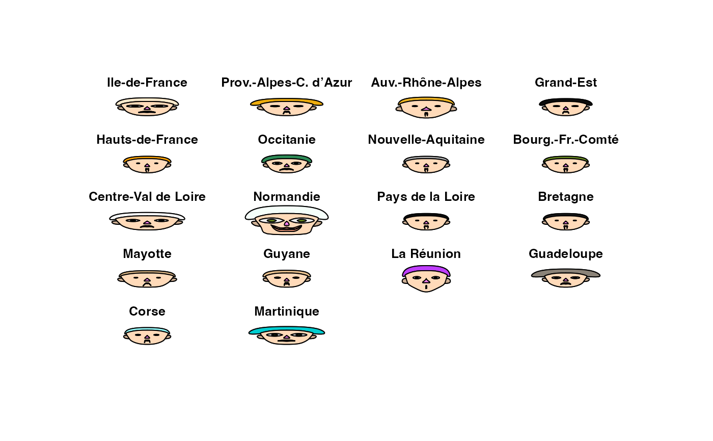
# print the used coding
print(z$info, right=FALSE)
#>    modified.item     variable
#> 1  height of face    X0.9
#> 2  width of face     X10.19
#> 3  structure of face X20.29
#> 4  height of mouth   X30.39
#> 5  width of mouth    X40.49
#> 6  smiling           X50.59
#> 7  height of eyes    X60.69
#> 8  width of eyes     X70.79
#> 9  height of hair    X80.89
#> 10 width of hair     X90.
#> 11 style of hair
#> 12 height of nose
#> 13 width of nose
#> 14 width of ear
#> 15 height of ear
Chemin <- "~/Documents/Recherche/DeBoeck/Graphes/Fichiers/"
colmodel="cmyk"
pdf(file = "ReaEffChernoff.pdf",
    width = 10, height = 7, onefile = TRUE, family = "Helvetica",
    title = "Probability or cumulative distribution graphs", paper = "special", colormodel = colmodel)
par(mar = c(3, 3, 1, 1) + 0.1, mgp = c(2, 1, 0))
PlotFaces(m, nr=5, nc=4, col=col,labels = namesXReg)
#> Warning in title(xnames[ind]): for 'Prov.-Alpes-C. d’Azur' in 'mbcsToSbcs': '
#> substituted for ’ (U+2019)
dev.off()
#> agg_png
#>       2
data(ReaFull)
Rea=cbind(Région=(ReaFull$Région)[-nrow(ReaFull)],ReaFull[-nrow(ReaFull),-c(1,2)]/((ReaFull$Tous.âges)[-nrow(ReaFull)]))
summary(Rea)
#>     Région               X0.9              X10.19             X20.29
#>  Length:18          Min.   :0.000000   Min.   :0.000000   Min.   :0.000000
#>  Class :character   1st Qu.:0.000000   1st Qu.:0.000000   1st Qu.:0.000000
#>  Mode  :character   Median :0.000000   Median :0.000000   Median :0.003981
#>                     Mean   :0.001737   Mean   :0.004848   Mean   :0.021250
#>                     3rd Qu.:0.000000   3rd Qu.:0.002691   3rd Qu.:0.010840
#>                     Max.   :0.019231   Max.   :0.047619   Max.   :0.285714
#>      X30.39             X40.49            X50.59           X60.69
#>  Min.   :0.000000   Min.   :0.00000   Min.   :0.0000   Min.   :0.0000
#>  1st Qu.:0.003058   1st Qu.:0.03269   1st Qu.:0.1116   1st Qu.:0.2155
#>  Median :0.017580   Median :0.04873   Median :0.1314   Median :0.2957
#>  Mean   :0.022158   Mean   :0.07943   Mean   :0.1431   Mean   :0.2689
#>  3rd Qu.:0.027389   3rd Qu.:0.06561   3rd Qu.:0.1785   3rd Qu.:0.3409
#>  Max.   :0.083333   Max.   :0.33333   Max.   :0.3333   Max.   :0.4167
#>      X70.79           X80.89             X90.
#>  Min.   :0.0000   Min.   :0.00000   Min.   :0.000000
#>  1st Qu.:0.3317   1st Qu.:0.07368   1st Qu.:0.000000
#>  Median :0.3384   Median :0.08238   Median :0.005284
#>  Mean   :0.3332   Mean   :0.07866   Mean   :0.018464
#>  3rd Qu.:0.3682   3rd Qu.:0.09979   3rd Qu.:0.011858
#>  Max.   :0.4340   Max.   :0.20000   Max.   :0.200000

means <- lapply(Rea[,-1], tapply, Rea$Région, mean)
m1 <- t(do.call(rbind, means))
# Complétion car au plus 15 variables
m <- cbind(m1, matrix(rep(1, (15-ncol(m1))*nrow(m1)), nrow=nrow(m1)))

namesXReg <- Rea$Région
namesXReg[3] <- "Auv.-Rhône-Alpes"
namesXReg[8] <- "Bourg.-Fr.-Comté"
namesXReg[2] <- "Prov.-Alpes-C. d’Azur"

# define the colors, first for all faces the same
col <- replicate(nrow(m1), c("orchid1", "olivedrab", "goldenrod4", "peachpuff", "darksalmon", "peachpuff3"))
rownames(col) <- c("nose","eyes","hair","face","lips","ears")
# change haircolor individually for each face
# col[3, ] <- c("lightgoldenrod", "coral3", "sienna4")
set.seed(4669)
col[3, ] <- sample(colors(),nrow(m1))
z <- PlotFaces(m, nr=5, nc=4, col=col,labels = namesXReg)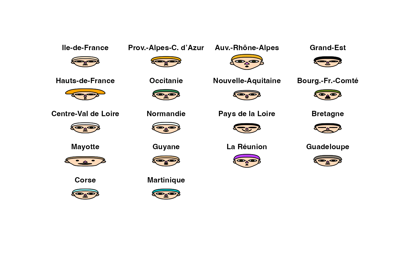
# print the used coding
print(z$info, right=FALSE)
#>    modified.item     variable
#> 1  height of face    X0.9
#> 2  width of face     X10.19
#> 3  structure of face X20.29
#> 4  height of mouth   X30.39
#> 5  width of mouth    X40.49
#> 6  smiling           X50.59
#> 7  height of eyes    X60.69
#> 8  width of eyes     X70.79
#> 9  height of hair    X80.89
#> 10 width of hair     X90.
#> 11 style of hair
#> 12 height of nose
#> 13 width of nose
#> 14 width of ear
#> 15 height of ear
Chemin <- "~/Documents/Recherche/DeBoeck/Graphes/Fichiers/"
colmodel="cmyk"
pdf(file = "ReaFreLignesChernoff.pdf",
    width = 10, height = 7, onefile = TRUE, family = "Helvetica",
    title = "Probability or cumulative distribution graphs", paper = "special", colormodel = colmodel)
par(mar = c(3, 3, 1, 1) + 0.1, mgp = c(2, 1, 0))
PlotFaces(m, nr=5, nc=4, col=col,labels = namesXReg)
#> Warning in title(xnames[ind]): for 'Prov.-Alpes-C. d’Azur' in 'mbcsToSbcs': '
#> substituted for ’ (U+2019)
dev.off()
#> agg_png
#>       2
data(HospitFull)
Hospit=cbind(Région=(HospitFull$Région)[-nrow(HospitFull)],HospitFull[-nrow(HospitFull),-c(1,2)])
summary(Hospit)
#>     Région               X0.9            X10.19           X20.29
#>  Length:18          Min.   : 0.000   Min.   : 0.000   Min.   : 0.00
#>  Class :character   1st Qu.: 0.000   1st Qu.: 0.000   1st Qu.: 3.00
#>  Mode  :character   Median : 1.000   Median : 2.500   Median : 9.00
#>                     Mean   : 2.222   Mean   : 4.278   Mean   :12.72
#>                     3rd Qu.: 2.000   3rd Qu.: 6.500   3rd Qu.:15.75
#>                     Max.   :17.000   Max.   :27.000   Max.   :72.00
#>      X30.39           X40.49           X50.59          X60.69
#>  Min.   :  0.00   Min.   :  0.00   Min.   :  2.0   Min.   :  2.00
#>  1st Qu.:  4.00   1st Qu.:  7.25   1st Qu.: 10.0   1st Qu.: 15.75
#>  Median : 15.00   Median : 28.00   Median : 81.0   Median :184.50
#>  Mean   : 23.89   Mean   : 43.83   Mean   :114.3   Mean   :232.28
#>  3rd Qu.: 34.25   3rd Qu.: 64.75   3rd Qu.:179.5   3rd Qu.:359.75
#>  Max.   :128.00   Max.   :192.00   Max.   :521.0   Max.   :861.00
#>      X70.79           X80.89            X90.
#>  Min.   :   5.0   Min.   :   1.0   Min.   :  0.0
#>  1st Qu.:  13.0   1st Qu.:  11.5   1st Qu.:  9.0
#>  Median : 296.0   Median : 418.0   Median :221.0
#>  Mean   : 376.1   Mean   : 494.3   Mean   :239.3
#>  3rd Qu.: 599.8   3rd Qu.: 798.0   3rd Qu.:382.5
#>  Max.   :1222.0   Max.   :1607.0   Max.   :783.0

means <- lapply(Hospit[,-1], tapply, Hospit$Région, mean)
m1 <- t(do.call(rbind, means))
# Complétion car au plus 15 variables
m <- cbind(m1, matrix(rep(1, (15-ncol(m1))*nrow(m1)), nrow=nrow(m1)))

namesXReg <- Rea$Région
namesXReg[3] <- "Auv.-Rhône-Alpes"
namesXReg[8] <- "Bourg.-Fr.-Comté"
namesXReg[2] <- "Prov.-Alpes-C. d’Azur"

# define the colors, first for all faces the same
col <- replicate(nrow(m1), c("orchid1", "olivedrab", "goldenrod4", "peachpuff", "darksalmon", "peachpuff3"))
rownames(col) <- c("nose","eyes","hair","face","lips","ears")
# change haircolor individually for each face
# col[3, ] <- c("lightgoldenrod", "coral3", "sienna4")
set.seed(4669)
col[3, ] <- sample(colors(),nrow(m1))
z <- PlotFaces(m, nr=5, nc=4, col=col,labels = namesXReg)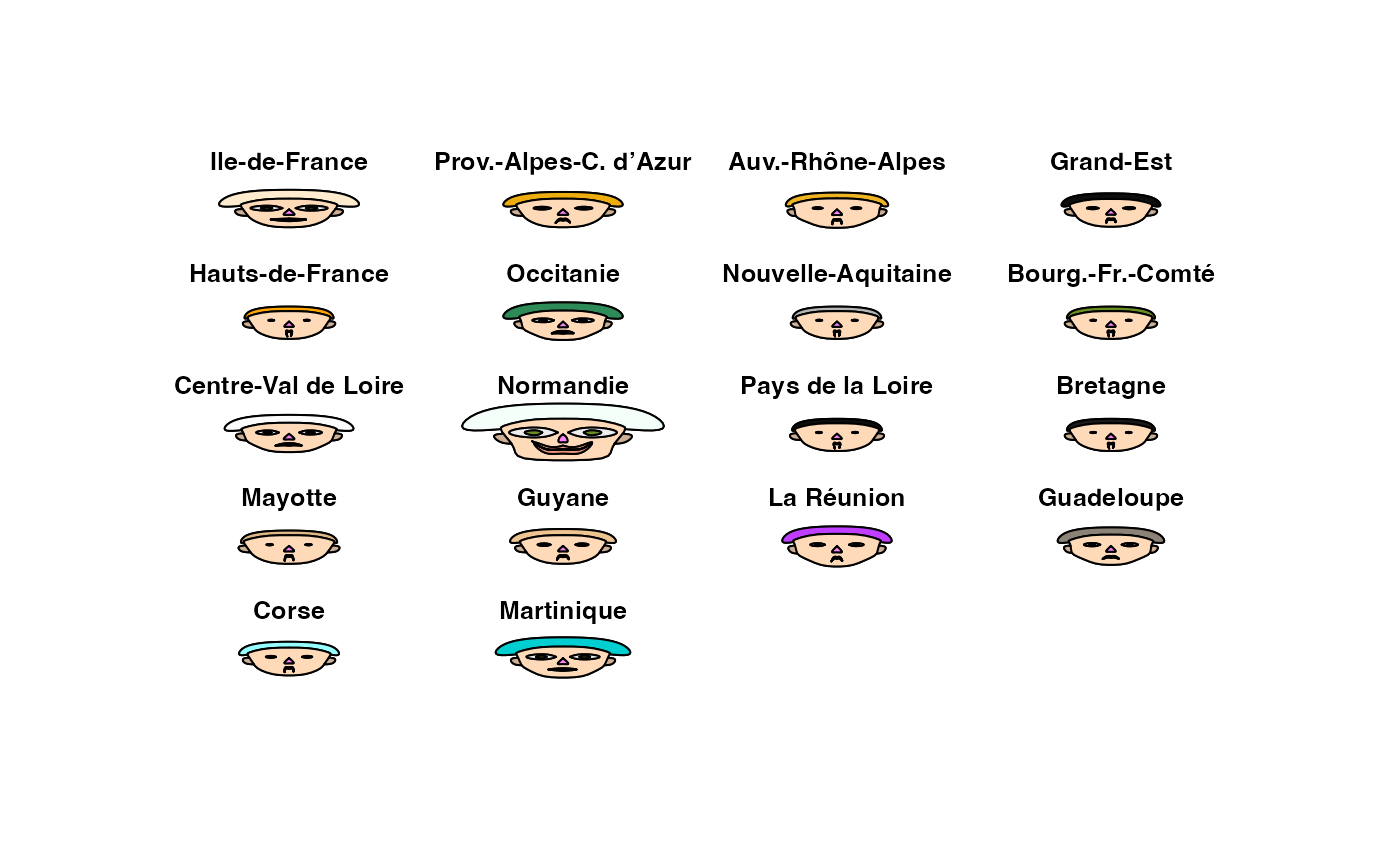
# print the used coding
print(z$info, right=FALSE)
#>    modified.item     variable
#> 1  height of face    X0.9
#> 2  width of face     X10.19
#> 3  structure of face X20.29
#> 4  height of mouth   X30.39
#> 5  width of mouth    X40.49
#> 6  smiling           X50.59
#> 7  height of eyes    X60.69
#> 8  width of eyes     X70.79
#> 9  height of hair    X80.89
#> 10 width of hair     X90.
#> 11 style of hair
#> 12 height of nose
#> 13 width of nose
#> 14 width of ear
#> 15 height of ear
Chemin <- "~/Documents/Recherche/DeBoeck/Graphes/Fichiers/"
colmodel="cmyk"
pdf(file = "HospitEffChernoff.pdf",
    width = 10, height = 7, onefile = TRUE, family = "Helvetica",
    title = "Probability or cumulative distribution graphs", paper = "special", colormodel = colmodel)
par(mar = c(3, 3, 1, 1) + 0.1, mgp = c(2, 1, 0))
PlotFaces(m, nr=5, nc=4, col=col,labels = namesXReg)
#> Warning in title(xnames[ind]): for 'Prov.-Alpes-C. d’Azur' in 'mbcsToSbcs': '
#> substituted for ’ (U+2019)
dev.off()
#> agg_png
#>       2
data(HospitFull)
Hospit=cbind(Région=(HospitFull$Région)[-nrow(HospitFull)],HospitFull[-nrow(HospitFull),-c(1,2)]/((HospitFull$Tous.âges)[-nrow(HospitFull)]))
summary(Hospit)
#>     Région               X0.9              X10.19             X20.29
#>  Length:18          Min.   :0.000000   Min.   :0.000000   Min.   :0.000000
#>  Class :character   1st Qu.:0.000000   1st Qu.:0.000000   1st Qu.:0.004985
#>  Mode  :character   Median :0.000644   Median :0.001690   Median :0.007432
#>                     Mean   :0.001380   Mean   :0.005508   Mean   :0.018862
#>                     3rd Qu.:0.001465   3rd Qu.:0.003730   3rd Qu.:0.012568
#>                     Max.   :0.009524   Max.   :0.047619   Max.   :0.152381
#>      X30.39             X40.49            X50.59            X60.69
#>  Min.   :0.000000   Min.   :0.00000   Min.   :0.04541   Min.   :0.1145
#>  1st Qu.:0.009531   1st Qu.:0.02308   1st Qu.:0.06561   1st Qu.:0.1367
#>  Median :0.011870   Median :0.02847   Median :0.06969   Median :0.1529
#>  Mean   :0.025165   Mean   :0.04494   Mean   :0.08996   Mean   :0.1718
#>  3rd Qu.:0.017364   3rd Qu.:0.03818   3rd Qu.:0.09344   3rd Qu.:0.1650
#>  Max.   :0.133333   Max.   :0.16190   Max.   :0.20000   Max.   :0.4412
#>      X70.79           X80.89             X90.
#>  Min.   :0.1143   Min.   :0.02857   Min.   :0.0000
#>  1st Qu.:0.2087   1st Qu.:0.21849   1st Qu.:0.1387
#>  Median :0.2384   Median :0.31125   Median :0.1506
#>  Mean   :0.2336   Mean   :0.26288   Mean   :0.1317
#>  3rd Qu.:0.2555   3rd Qu.:0.33508   3rd Qu.:0.1703
#>  Max.   :0.4167   Max.   :0.39487   Max.   :0.2679

means <- lapply(Hospit[,-1], tapply, Hospit$Région, mean)
m1 <- t(do.call(rbind, means))
# Complétion car au plus 15 variables
m <- cbind(m1, matrix(rep(1, (15-ncol(m1))*nrow(m1)), nrow=nrow(m1)))

namesXReg <- Rea$Région
namesXReg[3] <- "Auv.-Rhône-Alpes"
namesXReg[8] <- "Bourg.-Fr.-Comté"
namesXReg[2] <- "Prov.-Alpes-C. d’Azur"

# define the colors, first for all faces the same
col <- replicate(nrow(m1), c("orchid1", "olivedrab", "goldenrod4", "peachpuff", "darksalmon", "peachpuff3"))
rownames(col) <- c("nose","eyes","hair","face","lips","ears")
# change haircolor individually for each face
# col[3, ] <- c("lightgoldenrod", "coral3", "sienna4")
set.seed(4669)
col[3, ] <- sample(colors(),nrow(m1))
z <- PlotFaces(m, nr=5, nc=4, col=col,labels = namesXReg)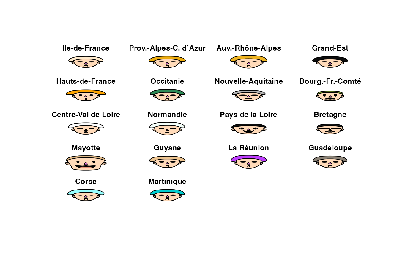
# print the used coding
print(z$info, right=FALSE)
#>    modified.item     variable
#> 1  height of face    X0.9
#> 2  width of face     X10.19
#> 3  structure of face X20.29
#> 4  height of mouth   X30.39
#> 5  width of mouth    X40.49
#> 6  smiling           X50.59
#> 7  height of eyes    X60.69
#> 8  width of eyes     X70.79
#> 9  height of hair    X80.89
#> 10 width of hair     X90.
#> 11 style of hair
#> 12 height of nose
#> 13 width of nose
#> 14 width of ear
#> 15 height of ear
Chemin <- "~/Documents/Recherche/DeBoeck/Graphes/Fichiers/"
colmodel="cmyk"
pdf(file = "HospitFreLignesChernoff.pdf",
    width = 10, height = 7, onefile = TRUE, family = "Helvetica",
    title = "Probability or cumulative distribution graphs", paper = "special", colormodel = colmodel)
par(mar = c(9.1, 3, 1, 1) + 0.1, mgp = c(2, 1, 0))
PlotFaces(m, nr=5, nc=4, col=col,labels = namesXReg)
#> Warning in title(xnames[ind]): for 'Prov.-Alpes-C. d’Azur' in 'mbcsToSbcs': '
#> substituted for ’ (U+2019)
dev.off()
#> agg_png
#>       2
Mesures de liaison
Salariés*Non-salariés (Quanti-Quanti)
data(Europe)

sum((Europe$Salariés-mean(Europe$Salariés))*(Europe$NonSalariés-mean(Europe$NonSalariés)))/nrow(Europe)
#> [1] 1.150155
cov(Europe$Salariés,Europe$NonSalariés)*(nrow(Europe)-1)/nrow(Europe)
#> [1] 1.150155
var(Europe$Salariés)*(nrow(Europe)-1)/nrow(Europe)
#> [1] 3.411478
var(Europe$NonSalariés)*(nrow(Europe)-1)/nrow(Europe)
#> [1] 9.449682
sum((Europe$Salariés-mean(Europe$Salariés))*(Europe$Salariés-mean(Europe$Salariés)))/nrow(Europe)
#> [1] 3.411478
sum((Europe$NonSalariés-mean(Europe$NonSalariés))*(Europe$NonSalariés-mean(Europe$NonSalariés)))/nrow(Europe)
#> [1] 9.449682

sqrt(sum((Europe$Salariés-mean(Europe$Salariés))*(Europe$Salariés-mean(Europe$Salariés)))/nrow(Europe))
#> [1] 1.847019
sqrt(sum((Europe$NonSalariés-mean(Europe$NonSalariés))*(Europe$NonSalariés-mean(Europe$NonSalariés)))/nrow(Europe))
#> [1] 3.074033

cov(Europe$Salariés,Europe$NonSalariés)*(nrow(Europe)-1)/nrow(Europe)/(sqrt(sum((Europe$Salariés-mean(Europe$Salariés))*(Europe$Salariés-mean(Europe$Salariés)))/nrow(Europe))*sqrt(sum((Europe$NonSalariés-mean(Europe$NonSalariés))*(Europe$NonSalariés-mean(Europe$NonSalariés)))/nrow(Europe)))
#> [1] 0.2025707
cor(Europe$Salariés,Europe$NonSalariés)
#> [1] 0.2025707
c(Europe$Partiel_Ens,Europe$Partiel_H,Europe$Partiel_F)
#>   [1] 27.2 27.2 24.9  1.9 10.2  4.8 24.2 14.5 11.3 15.5 17.5  9.1  4.4 19.7 21.5
#>  [16] 18.7  8.4  6.4 17.0  4.1 12.2  4.5 25.8 50.2  6.1  8.1  6.1 24.4  9.7  4.5
#>  [31]  8.4 22.5 38.0  6.3  9.9  9.9  9.5 10.5  1.7  6.3  3.1 15.3  6.8  7.1 10.1
#>  [46]  7.5  5.9  2.5 10.1 10.3  8.2  5.8  4.7  5.6  4.1  5.9  4.7 15.2 27.9  3.5
#>  [61]  5.4  6.0 10.8  8.9  2.9  4.8 13.4 17.1  2.8  6.6 46.7 47.1 41.0  2.1 14.6
#>  [76]  6.7 33.9 23.7 15.9 21.3 28.0 13.5  6.8 30.6 34.1 32.9 10.9  8.0 30.4  4.3
#>  [91] 21.4  4.1 37.7 75.2  9.3 10.9  6.2 39.4 10.6  6.5 12.7 32.5 61.7 10.6 17.0
factor(c(rep("Ensemble",length(Europe$Partiel_Ens)),rep("Hommes",length(Europe$Partiel_H)),rep("Femmes",length(Europe$Partiel_F))))
#>   [1] Ensemble Ensemble Ensemble Ensemble Ensemble Ensemble Ensemble Ensemble
#>   [9] Ensemble Ensemble Ensemble Ensemble Ensemble Ensemble Ensemble Ensemble
#>  [17] Ensemble Ensemble Ensemble Ensemble Ensemble Ensemble Ensemble Ensemble
#>  [25] Ensemble Ensemble Ensemble Ensemble Ensemble Ensemble Ensemble Ensemble
#>  [33] Ensemble Ensemble Ensemble Hommes   Hommes   Hommes   Hommes   Hommes
#>  [41] Hommes   Hommes   Hommes   Hommes   Hommes   Hommes   Hommes   Hommes
#>  [49] Hommes   Hommes   Hommes   Hommes   Hommes   Hommes   Hommes   Hommes
#>  [57] Hommes   Hommes   Hommes   Hommes   Hommes   Hommes   Hommes   Hommes
#>  [65] Hommes   Hommes   Hommes   Hommes   Hommes   Hommes   Femmes   Femmes
#>  [73] Femmes   Femmes   Femmes   Femmes   Femmes   Femmes   Femmes   Femmes
#>  [81] Femmes   Femmes   Femmes   Femmes   Femmes   Femmes   Femmes   Femmes
#>  [89] Femmes   Femmes   Femmes   Femmes   Femmes   Femmes   Femmes   Femmes
#>  [97] Femmes   Femmes   Femmes   Femmes   Femmes   Femmes   Femmes   Femmes
#> [105] Femmes
#> Levels: Ensemble Femmes Hommes

donnees = data.frame(Taux=c(Europe$Partiel_Ens,Europe$Partiel_H,Europe$Partiel_F),Type=factor(c(rep("Ensemble",length(Europe$Partiel_Ens)),rep("Hommes",length(Europe$Partiel_H)),rep("Femmes",length(Europe$Partiel_F)))))
tapply(donnees$Taux,donnees$Type,mean)
#>  Ensemble    Femmes    Hommes
#> 15.005714 23.094286  8.025714

var(tapply(donnees$Taux,donnees$Type,mean))*(nlevels(donnees$Type)-1)/nlevels(donnees$Type)
#> [1] 37.91191
mean(tapply(donnees$Taux,donnees$Type,var)*(length(Europe$Partiel_Ens)-1)/length(Europe$Partiel_Ens))
#> [1] 144.2113


var(tapply(donnees$Taux,donnees$Type,mean))*(nlevels(donnees$Type)-1)/nlevels(donnees$Type)+mean(tapply(donnees$Taux,donnees$Type,var))*(length(Europe$Partiel_Ens)-1)/length(Europe$Partiel_Ens)
#> [1] 182.1232
var(donnees$Taux)*(nlevels(donnees$Type)*length(Europe$Partiel_Ens)-1)/nlevels(donnees$Type)/length(Europe$Partiel_Ens)
#> [1] 182.1232

var(tapply(donnees$Taux,donnees$Type,mean))*(nlevels(donnees$Type)-1)/nlevels(donnees$Type)/(var(donnees$Taux)*(nlevels(donnees$Type)*length(Europe$Partiel_F)-1)/nlevels(donnees$Type)/length(Europe$Partiel_Ens))
#> [1] 0.2081663
Provinces et territoires vs Sexe Canada (Quali-Quali)
data(ProtervsSexe_Canada)Association
ProtervsSexe_Canada.table <- as.table(as.matrix(ProtervsSexe_Canada))
aaa=chisq.test(ProtervsSexe_Canada.table)
aaa$expected
#>                               Hommes     Femmes
#> Terre-Neuve-et-Labrador    259439.28  262663.72
#> Île-du-Prince-Édouard       79319.59   80305.41
#> Nouvelle-Écosse            486651.32  492699.68
#> Nouveau-Brunswick          388324.85  393151.15
#> Québec                    4260807.72 4313763.28
#> Ontario                   7321509.21 7412504.79
#> Manitoba                   685372.41  693890.59
#> Saskatchewan               585700.80  592980.20
#> Alberta                   2197283.50 2224592.50
#> Colombie-Britannique      2557960.16 2589751.84
#> Yukon                       20896.15   21155.85
#> Territoires du Nord-Ouest   22441.05   22719.95
#> Nunavut                     19554.98   19798.02
aaa$statistic
#> X-squared
#>  2152.457
aaa$statistic/(sum(ProtervsSexe_Canada.table))
#>    X-squared
#> 5.663581e-05
OCDE Secteur (Quali-Quali)
data(Secteur)

rownames(Secteur) <- Secteur$PAYS
Secteur <- as.table(as.matrix(round(Secteur[,-1]*1000)))

Secteur.table <- as.table(as.matrix(Secteur))
bbb=chisq.test(Secteur.table)
bbb$expected
#>             AGR      CONSTR  INDUSCONSTR          MFG         SERV
#> AUT  189776.809   315922.44   943693.373   577117.965   3311392.41
#> BEL  203404.049   338607.78  1011456.845   618558.880   3549172.45
#> CAN  750955.326  1250119.23  3734236.899  2283681.607  13103327.94
#> CHE  197989.374   329593.94   984531.571   602092.663   3454692.45
#> CHL  310449.251   516806.48  1543755.014   944087.112   5416991.14
#> COL  810284.374  1348884.60  4029259.407  2464103.335  14138553.28
#> CZE  249426.081   415220.89  1240308.237   758513.502   4352205.29
#> DNK  118862.206   197870.53   591059.972   361464.156   2074012.14
#> ESP  807113.679  1343606.33  4013492.652  2454461.138  14083228.20
#> EST    7119.071    11851.15    35400.636    21649.345    124219.80
#> FIN   41045.403    68328.49   204104.361   124820.516    716196.23
#> FRA 1129699.978  1880617.42  5617600.942  3435457.442  19711997.22
#> GBR 1328018.819  2210759.82  6603770.835  4038552.026  23172438.50
#> GRC  155792.242   259348.15   774700.064   473769.698   2718399.84
#> HUN  205766.098   342539.89  1023202.487   625741.956   3590387.57
#> IRL   95718.116   159342.44   475972.547   291082.162   1670173.73
#> ISL    1429.965     2380.47     7110.712     4348.573     24951.28
#> ISR  155249.708   258444.99   772002.233   472119.833   2708933.23
#> ITA 1010023.972  1681392.15  5022494.223  3071518.489  17623785.17
#> JPN 2914535.166  4851841.81 14492959.023  8863204.142  50855368.85
#> KOR 1182576.889  1968641.88  5880539.237  3596257.992  20634640.00
#> LTU   58572.345    97505.69   291259.687   178120.566   1022021.71
#> LUX   11266.256    18755.00    56023.133    34261.082    196583.53
#> LVA    9013.176    15004.28    44819.355    27409.385    157269.80
#> NLD  360634.361   600349.89  1793307.929  1096701.801   6292665.02
#> NOR  110723.448   184321.90   550588.793   336713.908   1931999.95
#> NZL  115284.218   191914.24   573267.900   350583.371   2011580.27
#> POL  746826.023  1243245.16  3713703.328  2271124.252  13031276.24
#> PRT  209835.175   349313.70  1043436.574   638116.160   3661388.39
#> SVK  120358.121   200360.79   598498.632   366013.286   2100114.17
#> SVN   45350.940    75495.95   225514.285   137913.806    791323.02
#> SWE  208774.496   347547.99  1038162.191   634890.598   3642880.73
#> TUR 1194746.433  1988900.59  5941054.099  3633266.003  20846984.88
#> USA 6086962.433 10132997.95 30268324.824 18510667.250 106210665.55
bbb$statistic
#> X-squared
#>  43415630
bbb$statistic/(sum(Secteur.table))
#>  X-squared
#> 0.07300288
Taux partiel ANOVA (Quali-Quanti)
data(Europe)

donnees = data.frame(Taux=c(Europe$Partiel_Ens,Europe$Partiel_H,Europe$Partiel_F),Type=factor(c(rep("Ensemble",nrow(Europe)),rep("Hommes",nrow(Europe)),rep("Femmes",nrow(Europe)))))
tapply(donnees$Taux,donnees$Type,mean)
#>  Ensemble    Femmes    Hommes
#> 15.005714 23.094286  8.025714

var(tapply(donnees$Taux,donnees$Type,mean))*(nlevels(donnees$Type)-1)/nlevels(donnees$Type)
#> [1] 37.91191
mean(tapply(donnees$Taux,donnees$Type,var)*(nrow(Europe)-1)/nrow(Europe))
#> [1] 144.2113


var(tapply(donnees$Taux,donnees$Type,mean))*(nlevels(donnees$Type)-1)/nlevels(donnees$Type)+mean(tapply(donnees$Taux,donnees$Type,var)*(nrow(Europe)-1)/nrow(Europe))
#> [1] 182.1232
var(donnees$Taux)*(nlevels(donnees$Type)*nrow(Europe)-1)/nlevels(donnees$Type)/nrow(Europe)
#> [1] 182.1232

var(tapply(donnees$Taux,donnees$Type,mean))*(nlevels(donnees$Type)-1)/nlevels(donnees$Type)/(var(donnees$Taux)*(nlevels(donnees$Type)*nrow(Europe)-1)/nlevels(donnees$Type)/nrow(Europe))
#> [1] 0.2081663

summary(lm(Taux~Type,data=donnees))
#>
#> Call:
#> lm(formula = Taux ~ Type, data = donnees)
#>
#> Residuals:
#>     Min      1Q  Median      3Q     Max
#> -20.994  -7.194  -2.026   6.494  52.106
#>
#> Coefficients:
#>             Estimate Std. Error t value Pr(>|t|)
#> (Intercept)   15.006      2.059   7.286 6.93e-11 ***
#> TypeFemmes     8.089      2.913   2.777  0.00653 **
#> TypeHommes    -6.980      2.913  -2.397  0.01837 *
#> ---
#> Signif. codes:  0 '***' 0.001 '**' 0.01 '*' 0.05 '.' 0.1 ' ' 1
#>
#> Residual standard error: 12.18 on 102 degrees of freedom
#> Multiple R-squared:  0.2082, Adjusted R-squared:  0.1926
#> F-statistic: 13.41 on 2 and 102 DF,  p-value: 6.766e-06
par(mar = c(2, 2, 1, 1) + 0.1, mgp = c(2, 1, 0))
pie(table(donnees$Type),labels=levels(donnees$Type),col=c("white","#00FFFF","black","#00FFFF"),border=c("black","#00FFFF","black","#00FFFF"),density=25,cex=1.2)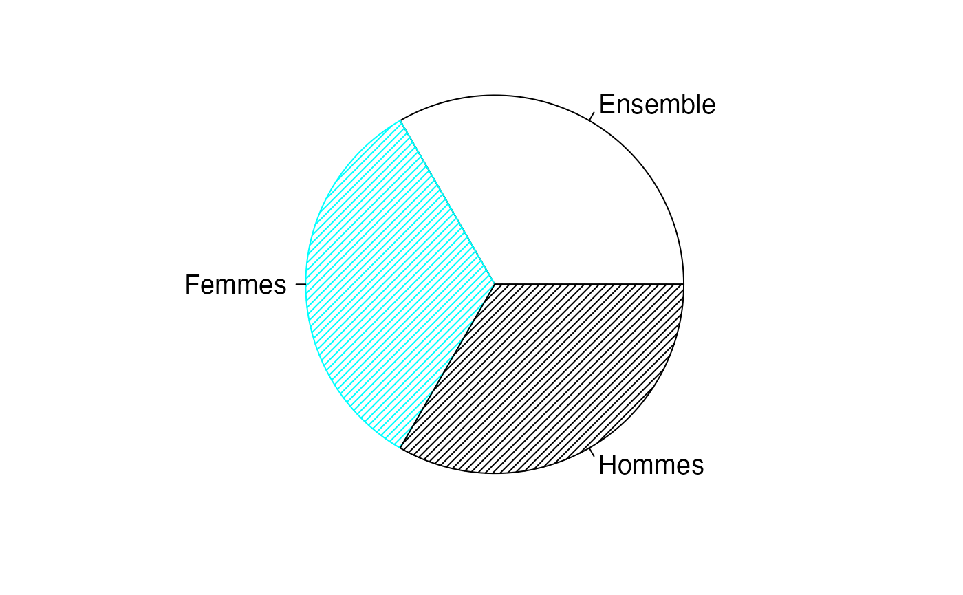
Chemin <- "~/Documents/Recherche/DeBoeck/Graphes/Fichiers/"
colmodel="cmyk"
pdf(file = "TauxEHF_qqualimarg_pie.pdf",
    width = 8, height = 7, onefile = TRUE, family = "Helvetica",
    title = "Probability or cumulative distribution graphs", paper = "special", colormodel = colmodel)
par(mar = c(2, 2, 1, 1) + 0.1, mgp = c(2, 1, 0))
pie(table(donnees$Type),labels=levels(donnees$Type),col=c("white","#00FFFF","black","#00FFFF"),border=c("black","#00FFFF","black","#00FFFF"),density=25,cex=1.2)
dev.off()
#> agg_png
#>       2

pdf(file = "TauxEHF_qqualimarg.pdf",
    width = 8, height = 7, onefile = TRUE, family = "Helvetica",
    title = "Probability or cumulative distribution graphs", paper = "special", colormodel = colmodel)
par(mar = c(2, 2, 1, 1) + 0.1, mgp = c(2, 1, 0))
dotplot(table(donnees$Type),labels=levels(donnees$Type),col=c("#00FFFF","#00FFFF","#00FFFF","#00FFFF"),border=c("#00FFFF","#00FFFF","#00FFFF","#00FFFF"),density=25,cex=1.2)
dev.off()
#> agg_png
#>       2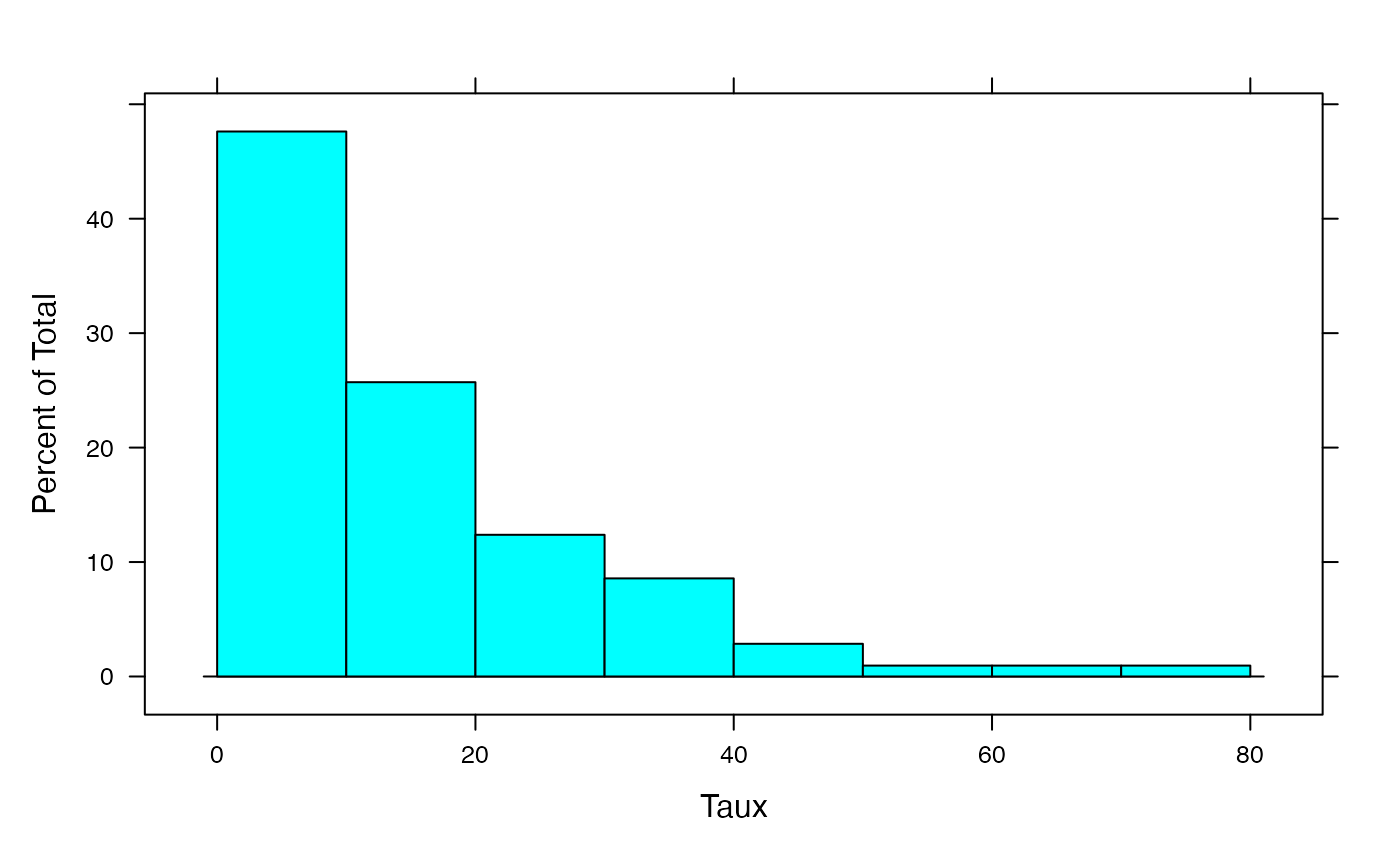
Chemin <- "~/Documents/Recherche/DeBoeck/Graphes/Fichiers/"
colmodel="cmyk"
pdf(file = "TauxEHF_qquantimarg.pdf",
    width = 8, height = 7, onefile = TRUE, family = "Helvetica",
    title = "Probability or cumulative distribution graphs", paper = "special", colormodel = colmodel)
par(mar = c(2, 2, 1, 1) + 0.1, mgp = c(2, 1, 0))
histogram(~Taux,data=donnees,breaks=c(0,10,20,30,40,50,60,70,80))
dev.off()
#> agg_png
#>       2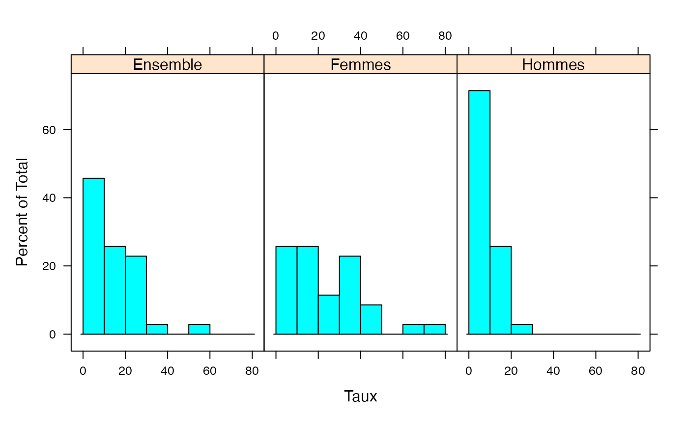
Chemin <- "~/Documents/Recherche/DeBoeck/Graphes/Fichiers/"
colmodel="cmyk"
pdf(file = "TauxEHF_qquanticond.pdf",
    width = 8, height = 7, onefile = TRUE, family = "Helvetica",
    title = "Probability or cumulative distribution graphs", paper = "special", colormodel = colmodel)
par(mar = c(2, 2, 1, 1) + 0.1, mgp = c(2, 1, 0))
histogram(~Taux|Type,data=donnees,breaks=c(0,10,20,30,40,50,60,70,80))
dev.off()
#> agg_png
#>       2
TauxQuali <- cut(donnees$Taux,c(0,10,20,30,40,50,60,70,80))
split(donnees$Type,TauxQuali)
#> $`(0,10]`
#>  [1] Ensemble Ensemble Ensemble Ensemble Ensemble Ensemble Ensemble Ensemble
#>  [9] Ensemble Ensemble Ensemble Ensemble Ensemble Ensemble Ensemble Ensemble
#> [17] Hommes   Hommes   Hommes   Hommes   Hommes   Hommes   Hommes   Hommes
#> [25] Hommes   Hommes   Hommes   Hommes   Hommes   Hommes   Hommes   Hommes
#> [33] Hommes   Hommes   Hommes   Hommes   Hommes   Hommes   Hommes   Hommes
#> [41] Hommes   Femmes   Femmes   Femmes   Femmes   Femmes   Femmes   Femmes
#> [49] Femmes   Femmes
#> Levels: Ensemble Femmes Hommes
#>
#> $`(10,20]`
#>  [1] Ensemble Ensemble Ensemble Ensemble Ensemble Ensemble Ensemble Ensemble
#>  [9] Ensemble Hommes   Hommes   Hommes   Hommes   Hommes   Hommes   Hommes
#> [17] Hommes   Hommes   Femmes   Femmes   Femmes   Femmes   Femmes   Femmes
#> [25] Femmes   Femmes   Femmes
#> Levels: Ensemble Femmes Hommes
#>
#> $`(20,30]`
#>  [1] Ensemble Ensemble Ensemble Ensemble Ensemble Ensemble Ensemble Ensemble
#>  [9] Hommes   Femmes   Femmes   Femmes   Femmes
#> Levels: Ensemble Femmes Hommes
#>
#> $`(30,40]`
#> [1] Ensemble Femmes   Femmes   Femmes   Femmes   Femmes   Femmes   Femmes
#> [9] Femmes
#> Levels: Ensemble Femmes Hommes
#>
#> $`(40,50]`
#> [1] Femmes Femmes Femmes
#> Levels: Ensemble Femmes Hommes
#>
#> $`(50,60]`
#> [1] Ensemble
#> Levels: Ensemble Femmes Hommes
#>
#> $`(60,70]`
#> [1] Femmes
#> Levels: Ensemble Femmes Hommes
#>
#> $`(70,80]`
#> [1] Femmes
#> Levels: Ensemble Femmes Hommes
sapply(split(donnees$Type,TauxQuali),table)
#>          (0,10] (10,20] (20,30] (30,40] (40,50] (50,60] (60,70] (70,80]
#> Ensemble     16       9       8       1       0       1       0       0
#> Femmes        9       9       4       8       3       0       1       1
#> Hommes       25       9       1       0       0       0       0       0

regroup <- sapply(split(donnees$Type,TauxQuali),table)
par(mar = c(3, 3, 1, 1) + 0.1, mgp = c(2, 1, 0))
barplot(regroup,beside=TRUE, legend=levels(donnees$Type), args.legend=list(x="topright", ncol=1))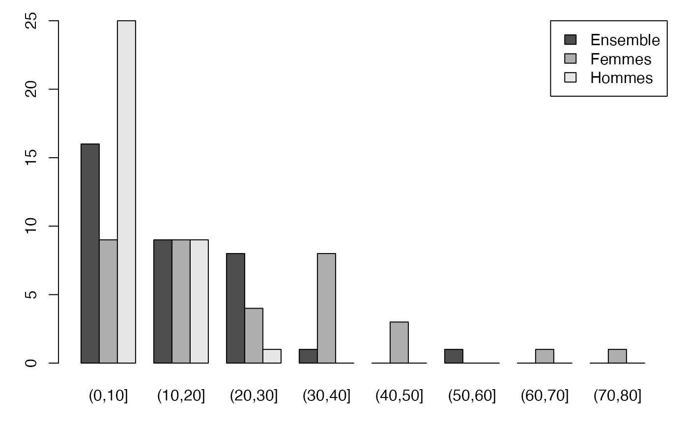
Chemin <- "~/Documents/Recherche/DeBoeck/Graphes/Fichiers/"
colmodel="cmyk"
pdf(file = "TauxEHF_qqualicond.pdf",
    width = 8, height = 7, onefile = TRUE, family = "Helvetica",
    title = "Probability or cumulative distribution graphs", paper = "special", colormodel = colmodel)
par(mar = c(3, 3, 1, 1) + 0.1, mgp = c(2, 1, 0))
barplot(regroup,beside=TRUE, legend=levels(donnees$Type), args.legend=list(x="topright", ncol=1))
dev.off()
#> agg_png
#>       2
Iris Fisher (Quali-Quanti)
tapply(donnees$Sepal.Length,donnees$Species,mean)
#>     setosa versicolor  virginica
#>      5.006      5.936      6.588

var(tapply(donnees$Sepal.Length,donnees$Species,mean))*(nlevels(donnees$Species)-1)/nlevels(donnees$Species)
#> [1] 0.4214142
mean(tapply(donnees$Sepal.Length,donnees$Species,var)*(nrow(Europe)-1)/nrow(Europe))
#> [1] 0.2574365


var(tapply(donnees$Sepal.Length,donnees$Species,mean))*(nlevels(donnees$Species)-1)/nlevels(donnees$Species)+mean(tapply(donnees$Sepal.Length,donnees$Species,var)*(nrow(Europe)-1)/nrow(Europe))
#> [1] 0.6788507
var(donnees$Sepal.Length)*(nlevels(donnees$Species)*nrow(Europe)-1)/nlevels(donnees$Species)/nrow(Europe)
#> [1] 0.6791631

var(tapply(donnees$Sepal.Length,donnees$Species,mean))*(nlevels(donnees$Species)-1)/nlevels(donnees$Species)/(var(donnees$Sepal.Length)*(nlevels(donnees$Species)*nrow(Europe)-1)/nlevels(donnees$Species)/nrow(Europe))
#> [1] 0.6204905

summary(lm(Sepal.Length~Species,data=donnees))
#>
#> Call:
#> lm(formula = Sepal.Length ~ Species, data = donnees)
#>
#> Residuals:
#>     Min      1Q  Median      3Q     Max
#> -1.6880 -0.3285 -0.0060  0.3120  1.3120
#>
#> Coefficients:
#>                   Estimate Std. Error t value Pr(>|t|)
#> (Intercept)         5.0060     0.0728  68.762  < 2e-16 ***
#> Speciesversicolor   0.9300     0.1030   9.033 8.77e-16 ***
#> Speciesvirginica    1.5820     0.1030  15.366  < 2e-16 ***
#> ---
#> Signif. codes:  0 '***' 0.001 '**' 0.01 '*' 0.05 '.' 0.1 ' ' 1
#>
#> Residual standard error: 0.5148 on 147 degrees of freedom
#> Multiple R-squared:  0.6187, Adjusted R-squared:  0.6135
#> F-statistic: 119.3 on 2 and 147 DF,  p-value: < 2.2e-16
par(mar = c(2, 2, 1, 1) + 0.1, mgp = c(2, 1, 0))
pie(table(donnees$Species),labels=levels(donnees$Species),col=c("white","#00FFFF","black","#00FFFF"),border=c("black","#00FFFF","black","#00FFFF"),density=25,cex=1.2)
Chemin <- "~/Documents/Recherche/DeBoeck/Graphes/Fichiers/"
colmodel="cmyk"
pdf(file = "Sepal.Length_iris_qqualimarg_pie.pdf",
    width = 8, height = 7, onefile = TRUE, family = "Helvetica",
    title = "Probability or cumulative distribution graphs", paper = "special", colormodel = colmodel)
par(mar = c(2, 2, 1, 1) + 0.1, mgp = c(2, 1, 0))
pie(table(donnees$Species),labels=levels(donnees$Species),col=c("white","#00FFFF","black","#00FFFF"),border=c("black","#00FFFF","black","#00FFFF"),density=25,cex=1.2)
dev.off()
#> agg_png
#>       2

pdf(file = "Sepal.Length_iris_qqualimarg.pdf",
    width = 8, height = 7, onefile = TRUE, family = "Helvetica",
    title = "Probability or cumulative distribution graphs", paper = "special", colormodel = colmodel)
par(mar = c(2, 2, 1, 1) + 0.1, mgp = c(2, 1, 0))
dotplot(table(donnees$Species),labels=levels(donnees$Species),col=c("#00FFFF","#00FFFF","#00FFFF","#00FFFF"),border=c("#00FFFF","#00FFFF","#00FFFF","#00FFFF"),density=25,cex=1.2)
dev.off()
#> agg_png
#>       2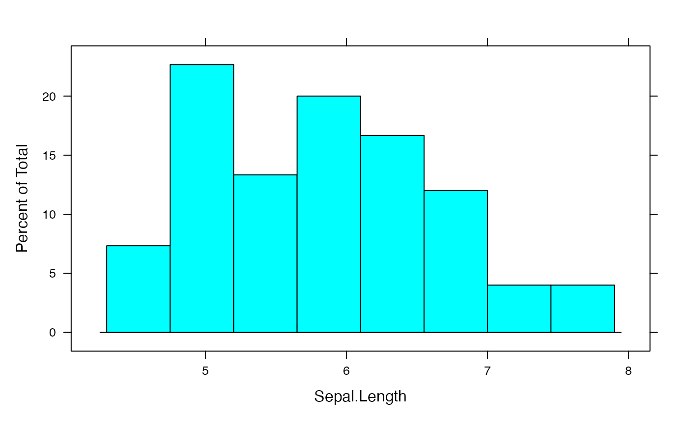
Chemin <- "~/Documents/Recherche/DeBoeck/Graphes/Fichiers/"
colmodel="cmyk"
pdf(file = "Sepal.Length_iris_qquantimarg.pdf",
    width = 8, height = 7, onefile = TRUE, family = "Helvetica",
    title = "Probability or cumulative distribution graphs", paper = "special", colormodel = colmodel)
par(mar = c(2, 2, 1, 1) + 0.1, mgp = c(2, 1, 0))
histogram(~Sepal.Length,data=donnees,breaks=c(4.3,4.75,5.2,5.65,6.1,6.55,7,7.45,7.9))
dev.off()
#> agg_png
#>       2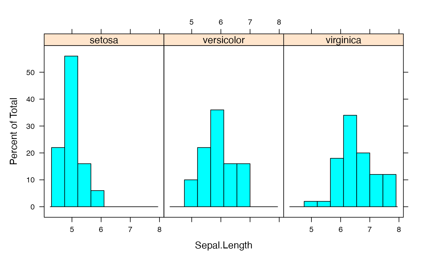
Chemin <- "~/Documents/Recherche/DeBoeck/Graphes/Fichiers/"
colmodel="cmyk"
pdf(file = "Sepal.Length_iris_qquanticond.pdf",
    width = 8, height = 7, onefile = TRUE, family = "Helvetica",
    title = "Probability or cumulative distribution graphs", paper = "special", colormodel = colmodel)
par(mar = c(2, 2, 1, 1) + 0.1, mgp = c(2, 1, 0))
histogram(~Sepal.Length|Species,data=donnees,breaks=c(4.3,4.75,5.2,5.65,6.1,6.55,7,7.45,7.9))
dev.off()
#> agg_png
#>       2
Sepal.LengthQuali <- cut(donnees$Sepal.Length,c(4.3,4.75,5.2,5.65,6.1,6.55,7,7.45,7.9))
split(donnees$Species,Sepal.LengthQuali)
#> $`(4.3,4.75]`
#>  [1] setosa setosa setosa setosa setosa setosa setosa setosa setosa setosa
#> Levels: setosa versicolor virginica
#>
#> $`(4.75,5.2]`
#>  [1] setosa     setosa     setosa     setosa     setosa     setosa
#>  [7] setosa     setosa     setosa     setosa     setosa     setosa
#> [13] setosa     setosa     setosa     setosa     setosa     setosa
#> [19] setosa     setosa     setosa     setosa     setosa     setosa
#> [25] setosa     setosa     setosa     setosa     versicolor versicolor
#> [31] versicolor versicolor versicolor virginica
#> Levels: setosa versicolor virginica
#>
#> $`(5.2,5.65]`
#>  [1] setosa     setosa     setosa     setosa     setosa     setosa
#>  [7] setosa     setosa     versicolor versicolor versicolor versicolor
#> [13] versicolor versicolor versicolor versicolor versicolor versicolor
#> [19] versicolor virginica
#> Levels: setosa versicolor virginica
#>
#> $`(5.65,6.1]`
#>  [1] setosa     setosa     setosa     versicolor versicolor versicolor
#>  [7] versicolor versicolor versicolor versicolor versicolor versicolor
#> [13] versicolor versicolor versicolor versicolor versicolor versicolor
#> [19] versicolor versicolor versicolor virginica  virginica  virginica
#> [25] virginica  virginica  virginica  virginica  virginica  virginica
#> Levels: setosa versicolor virginica
#>
#> $`(6.1,6.55]`
#>  [1] versicolor versicolor versicolor versicolor versicolor versicolor
#>  [7] versicolor versicolor virginica  virginica  virginica  virginica
#> [13] virginica  virginica  virginica  virginica  virginica  virginica
#> [19] virginica  virginica  virginica  virginica  virginica  virginica
#> [25] virginica
#> Levels: setosa versicolor virginica
#>
#> $`(6.55,7]`
#>  [1] versicolor versicolor versicolor versicolor versicolor versicolor
#>  [7] versicolor versicolor virginica  virginica  virginica  virginica
#> [13] virginica  virginica  virginica  virginica  virginica  virginica
#> Levels: setosa versicolor virginica
#>
#> $`(7,7.45]`
#> [1] virginica virginica virginica virginica virginica virginica
#> Levels: setosa versicolor virginica
#>
#> $`(7.45,7.9]`
#> [1] virginica virginica virginica virginica virginica virginica
#> Levels: setosa versicolor virginica
sapply(split(donnees$Species,Sepal.LengthQuali),table)
#>            (4.3,4.75] (4.75,5.2] (5.2,5.65] (5.65,6.1] (6.1,6.55] (6.55,7]
#> setosa             10         28          8          3          0        0
#> versicolor          0          5         11         18          8        8
#> virginica           0          1          1          9         17       10
#>            (7,7.45] (7.45,7.9]
#> setosa            0          0
#> versicolor        0          0
#> virginica         6          6

regroup <- sapply(split(donnees$Species,Sepal.LengthQuali),table)
par(mar = c(3, 3, 1, 1) + 0.1, mgp = c(2, 1, 0))
barplot(regroup,beside=TRUE, legend=levels(donnees$Species), args.legend=list(x="topright", ncol=1))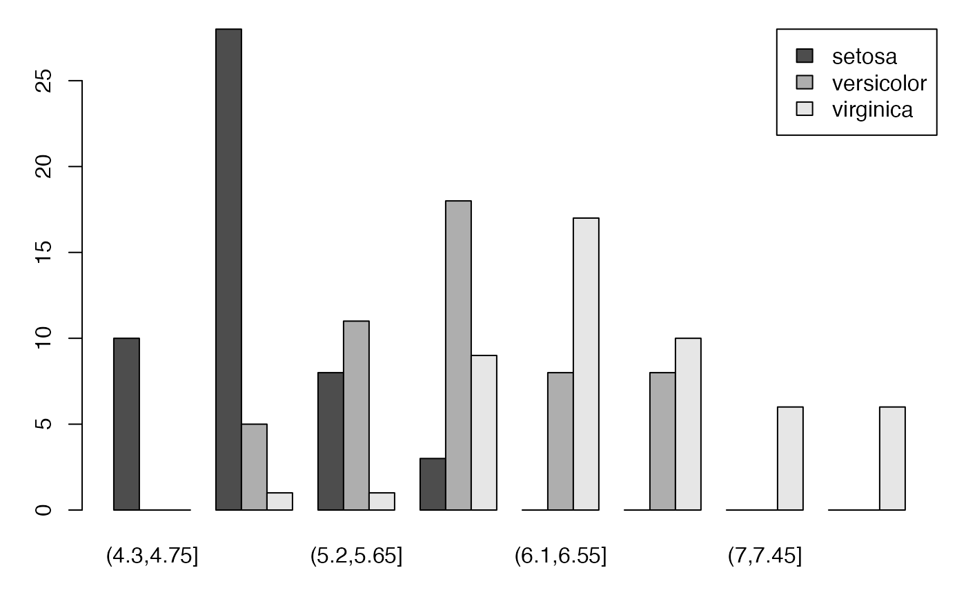
Chemin <- "~/Documents/Recherche/DeBoeck/Graphes/Fichiers/"
colmodel="cmyk"
pdf(file = "Sepal.Length_iris_qqualicond.pdf",
    width = 8, height = 7, onefile = TRUE, family = "Helvetica",
    title = "Probability or cumulative distribution graphs", paper = "special", colormodel = colmodel)
par(mar = c(3, 3, 1, 1) + 0.1, mgp = c(2, 1, 0))
barplot(regroup,beside=TRUE, legend=levels(donnees$Species), args.legend=list(x="topright", ncol=1))
dev.off()
#> agg_png
#>       2